Causal Estimation methods for Machine learning and Data Science Part III – Instrument Variable Analysis

1.0 Introduction

In the past two blogs of this series we’ve been discussing causal estimation, a very important subject in data science, we delved into causal estimation using regression method and propensity score matching. Now, let’s venture into the world of instrumental variable analysis—a powerful method for unearthing causal relationships from observational data. Let us look at the structure of this blog.

2.0 Structure

Instrument variables – An introduction
Instrument variable analysis – The process
Implementation of instrument variable analysis from scratch using linear regression
Implementation of instrument variable analysis using DoWhy
Implementation of instrument variable analysis using Ordinary Least Squares (OLS) Method
Conclusion

3.0 Instrument Variables – An introduction

Let us start the explanation on the instrument variable analysis with an example.

We all know education is important, but figuring out how much it REALLY boosts your future earnings is tricky. Its not easy to tell how big a difference an extra year of school makes because we also don’t know how smart someone already is. Some people are just naturally good at stuff, and that might be why they earn more, not just because they went to school longer. This confusing mix makes it hard to see the true effect of education.

But there’s a way out of this impasse!!

Imagine that you have a mechanism to separate the real link between education and earnings while ignoring how smart someone is. That’s what an instrument variable is. It helps us see the clear path between education and income, without getting fooled by other factors. In our example, an instrument variable that could be considered could be something like compulsory schooling laws. These laws force everyone to spend a certain amount of time in school, regardless of their natural talent. So, by studying how those laws affect people’s earnings, we can get a clearer picture of what education itself does, apart from just naturally-smart people earning more.

With this tool, we can finally answer the big question: is education really the key to unlocking a brighter financial future?

4.0 Instrument variable analysis – The process

Here’s how it works:

Effect of instrument on treatment: We analyze how compulsory schooling laws (the instrument variable) affect education (the treatment).
Estimate the effect of education on outcome: We use the information from the above to estimate how education (treatment) actually affects earnings (outcome), ignoring the influence of natural talent (the unobserved confounders).

By using this method, we can finally isolate the true effect of education on earnings, leaving the confusing influence of natural talent behind. Now, we can confidently answer the question:

Does more education truly lead to a brighter financial future?

Remember, this is just one example, and finding the right instrument variable for your situation can be tricky. But with the right tool in hand, you can navigate the maze of confounding factors and uncover the true causal relationships in your data.

Implementation of Causal estimation using Instrument Variables from scratch

Let us now explain the concept through code. First we will use the linear regression method to take you through the estimation process.

To start off, lets generate some synthetic data set which describes the relationship between the variables.

# Importing the necessary packages
import numpy as np
from sklearn.linear_model import LinearRegression

Now let’s create the synthetic dataset

# Generate sample data (replace with your actual data)
n = 1000
ability = np.random.normal(size=n)
compulsory_schooling = np.random.binomial(1, 0.5, size=n)
education = 5 + 2 * compulsory_schooling + 0.5 * ability + np.random.normal(size=n)
earnings = 10 + 3 * education + 0.8 * ability + np.random.normal(size=n)

This section creates simulated data for n individuals (1000 in this case):

ability: Represents unobserved individual ability (normally distributed).
compulsory_schooling: Binary variable indicating whether someone was subject to compulsory schooling (50% chance).
education: Years of education, determined by compulsory schooling (2 years difference), ability (0.5 years per unit), and random error.
earnings: Annual earnings, influenced by education (3 units per year), ability (0.8 units per unit), and random error.

We can see that the variables are defined in such a way that education depends on both schooling laws ( instrument variable) and ability ( unobserved confounder) and the earnings ( outcome ) depends on education ( Treatment ) and ability. The outcome is not directly influenced by the instrument variable, which is one of the condition of selecting an instrument variable.

Let us now implement the first regression model.

# Stage 1: Regress treatment (education) on instrument (compulsory schooling)
stage1_model = LinearRegression()
stage1_model.fit(compulsory_schooling.reshape(-1, 1), education)  # Reshape for 2D input
predicted_education = stage1_model.predict(compulsory_schooling.reshape(-1, 1))

This stage uses linear regression to model how compulsory schooling (compulsory_schooling) affects education (education).

In line 13, we reshape the data to the required 2D format for scikit-learn’s LinearRegression model. The model estimates the effect of compulsory schooling on education, isolating the variation in education directly caused by the instrument (compulsory schooling) and removing the influence of ability (confounding variable).

In line 14, The resulting model predicts the “purified” education values (predicted_education) for each individual, eliminating the confounding influence of ability.

Now that we have found the education variable which is precluded of the influence from unobserved confounder ( ability ), we will build the second regression model.

# Stage 2: Regress outcome (earnings) on predicted treatment from stage 1
stage2_model = LinearRegression()
stage2_model.fit(predicted_education.reshape(-1, 1), earnings)  # Reshape for 2D input

This stage uses linear regression to model how the predicted education (predicted_education) affects earnings (earnings).

Again, in line 16 we reshape the data for compatibility with the model and fit the model to estimate the causal effect of education on earnings. Here we use the “cleaned” education values from stage 1 to isolate the true effect, holding the influence of ability constant.

Let us now extract the coefficients of this model. The coefficient of predicted_education represents the estimated change in earnings associated with a one-unit increase in education, adjusting for the confounding effect of ability.

# Print coefficients (equivalent to summary in statsmodels)
print("Intercept:", stage2_model.intercept_)
print("Coefficient of education:", stage2_model.coef_[0])

Intercept (9.901): This indicates the predicted earnings for someone with zero years of education.

Coefficient of education (3.004): This shows that, on average, each additional year of education is associated with an increase of $3.004 in annual earnings, holding ability constant with the help of the instrument.

Let us try to get some intuition on the exercise we just performed. In the first stage, we estimate how changes in the instrument (here, compulsory schooling laws) impact education. Then in the second stage, we examine how changes in education, predicted from the first stage, impact earnings. The first stage helps address the issue of unobserved confounding by using a variable (the instrument) that only affects the outcome through its impact on the treatment variable. Thus we are able to estimate the real effect of education on the earning capacity, by eliminating any influence from the unobserved confounding variables like ability.

We implemented this exercise using linear regression to get an intuitive understanding of what is going on under the hood. Now let us implement the same exercise using DoWhy library.

5.0 Implementation using DoWhy

We will start by importing the required libraries.

from dowhy import CausalModel

We will be using the same data frame which we used earlier. Let us now define the data frame for our analysis.

# Create a pandas DataFrame
data = pd.DataFrame({
    'ability': ability,
    'compulsory_schooling': compulsory_schooling,
    'education': education,
    'earnings': earnings
})

Next let us define the causal model.

# Define the causal model
model = CausalModel(
    data=data,
    treatment='education',
    outcome='earnings',
    instruments=['compulsory_schooling']
)

The above code creates the causal model using DoWhy.

Let’s break down the key components and the processes happening behind the scenes:

model = CausalModel(...): This line initializes a causal model using the DoWhy library.

data: The dataset containing the variables of interest.

treatment='education': Specifies the treatment variable, i.e., the variable that is believed to have a causal effect on the outcome.

outcome='earnings': Specifies the outcome variable, i.e., the variable whose changes we want to attribute to the treatment.

instruments=['compulsory_schooling']: Specifies the instrumental variable(s), if any. In this case, ‘compulsory_schooling’ is used as an instrument.

In the provided code snippet, there is no explicit specification of common causes, which in our case is the variable ‘ability’. The absence of common causes in the CausalModel definition may imply that the common causes are either not considered or are left unspecified. In our case we have said that the common causes or confounders are unobserved. That is why we use the instrument variable ( compulsory_schooling) to negate the effect of unobserved confounders.

When the causal model is defined as shown above, DoWhy performs an identification step where it tries to identify the causal effect using graphical models and do-calculus. It checks if the causal effect is identifiable given the specified variables. To know more about the identification steps you can refer our previous blogs on the subject.

Once identification is successful, the next step is to estimate the causal effect. Let us proceed with the estimation process.

# Identify the causal effect using instrumental variable analysis
identified_estimand = model.identify_effect(proceed_when_unidentifiable=True)
estimate = model.estimate_effect(identified_estimand, method_name="iv.instrumental_variable")

Line 17 , identified_estimand = model.identify_effect(proceed_when_unidentifiable=True): In this step, the identify_effect method attempts to identify the causal effect based on the specified causal model. The proceed_when_unidentifiable=True parameter allows the analysis to proceed even if the causal effect is unidentifiable, with the understanding that this might result in less precise estimates.

Line 18 estimate = model.estimate_effect(identified_estimand, method_name="iv.instrumental_variable"): This method takes the identified estimand and specifies the method for estimating the causal effect. In this case, the method chosen is instrumental variable analysis, specified by method_name="iv.instrumental_variable". Instrumental variable analysis helps in addressing potential confounding in observational studies by finding an instrument (a variable that is correlated with the treatment but not directly associated with the outcome) to isolate the causal effect.The intuition for the instrument variable was earlier described when we built the linear regression model.

Finally the estimate object contains information about the estimated causal effect. Let us print the causal effect in our case

# Print the causal effect estimate
print("Causal Effect Estimate:", estimate.value)

From the output we can see that its similar to our implementation using the linear regression method. The idea of implementing the linear regression method is to unravel the intuition which is often hidden in black box implementations like that in the DoWhy package.

Now that we have a fair idea and intuition on what is happening in the instrument variable analysis, let us see one more method of implementation called the two-stage least squares (2SLS) regression method. We will be using the statsmodels library for the implementation.

6.0 Ordinary Least Squares (OLS) Method method

Let us see the full implementation using least squares method.

import numpy as np
import pandas as pd
import statsmodels.api as sm

# Set seed for reproducibility
np.random.seed(42)

# Generate synthetic data
n_samples = 1000

# True coefficients
beta_education = 3.5  # True causal effect of education on earnings
gamma_instrument = 2.0  # True effect of the instrument on education
delta_intercept = 5.0  # Intercept in the second stage equation

# Generate data
instrument_z = np.random.randint(0, 2, size=n_samples)  # Instrument (0 or 1)
education_x = 2 * instrument_z + np.random.normal(0, 1, n_samples)  # Education affected by the instrument
earnings_y = delta_intercept + beta_education * education_x + gamma_instrument * instrument_z + np.random.normal(0, 1, n_samples)

# Create a DataFrame
data = pd.DataFrame({'Education': education_x, 'Earnings': earnings_y, 'Instrument': instrument_z})

# First stage regression: Regress education on the instrument
first_stage = sm.OLS(data['Education'], sm.add_constant(data['Instrument'])).fit()
data['Predicted_Education'] = first_stage.predict()

# Second stage regression: Regress earnings on the predicted education
second_stage = sm.OLS(data['Earnings'], sm.add_constant(data['Predicted_Education'])).fit()

In line 6, we set the seed for reproducibility. Then in lines 12-14, we define the true coefficients for the simulation. This step is done only to compare the final results with the actual coefficients, since we have the luxury of defining the data itself.

In lines 17-19, we generate synthetic data for the analysis. The variables for this data are the following.

instrument_z represents the instrument (0 or 1).
education_x is affected by the instrument.
earnings_y is generated based on the true coefficients and some random noise.

In line 22, we create a DataFrame to hold the simulated data.

In lines 25-26, we perform the first stage regression: regress education on the instrument.

sm.OLS: This is creating an Ordinary Least Squares (OLS) regression model. OLS is a method for estimating the parameters in a linear regression model.
data['Education']: This is specifying the dependent variable in the regression, which is education (X).
sm.add_constant(data['Instrument']): This part is adding a constant term to the independent variable, which is the instrument (Z). The constant term represents the intercept in the linear regression equation.
.fit(): This fits the model to the data, estimating the coefficients.

We finally store the predictions in a variable ‘Predicted_Eduction‘

In the second stage regression in line 29, earnings is regressed on the predicted education from the first stage.This stage estimates the causal effect of education on earnings, considering the predicted education from the first stage.The coefficient of the predicted education in the second stage represents the causal effect.

Let us look at the results from each stage .

# Print results
print("First Stage Results:")
print(first_stage.summary())

print("\nSecond Stage Results:")
print(second_stage.summary())

Let’s interpret the results obtained from both the first and second stages:

First stage results:

Constant (Intercept): The constant term (const) is estimated to be 0.0462, but its p-value (P>|t|) is 0.308, indicating that it is not statistically significant. This suggests that the instrument is not systematically related to the baseline level of education.

Instrument: The coefficient for the instrument is 1.9882, and its p-value is very close to zero (P>|t| < 0.001). This implies that the instrument is statistically significant in predicting education.

R-squared: The R-squared value of 0.497 indicates that approximately 49.7% of the variability in education is explained by the instrument.

F-statistic:The F-statistic (984.4) is highly significant with a p-value close to zero. This suggests that the instrument as a whole is statistically significant in predicting education.

The overall fit of the first stage regression is reasonably good, given the significant F-statistic and the instrument’s significant coefficient.

The coefficient for the instrument (Z) being 1.9882 with a very low p-value suggests a statistically significant relationship between the instrument (compulsory schooling laws) and education (X). In the context of instrumental variable analysis, this implies that the instrument is a good predictor of the endogenous variable (education) and helps address the issue of endogeneity.

The compulsory schooling laws (instrument) affect education levels. The positive coefficient suggests that when these laws are in place, education levels tend to increase. This aligns with the intuition that compulsory schooling laws, which mandate individuals to stay in school for a certain duration, positively influence educational attainment.

In the context of the broader problem—examining whether education causally increases earnings—the significance of the instrument is crucial. It indicates that the laws that mandate schooling have a significant impact on the educational levels of individuals in the dataset. This, in turn, supports the validity of the instrument for addressing the potential endogeneity of education in the relationship with earnings.

Second stage results:

Constant (Intercept): The constant term (const) is estimated to be 5.0101, and it is statistically significant (P>|t| < 0.001). This represents the baseline earnings when the predicted education is zero.

Predicted Education: The coefficient for predicted education is 4.4884, and it is highly significant (P>|t| < 0.001). This implies that, controlling for the instrument, the predicted education has a positive effect on earnings.

R-squared: The R-squared value of 0.605 indicates that approximately 60.5% of the variability in earnings is explained by the predicted education.

F-statistic: The F-statistic (1530.0) is highly significant, suggesting that the model as a whole is statistically significant in predicting earnings.

The overall fit of the second stage regression is good, with significant coefficients for the constant and predicted education.

The coefficient for predicted education is 4.4884, and its high level of significance (P>|t| < 0.001) indicates that predicted education has a statistically significant and positive effect on earnings. In the second stage of instrumental variable analysis, predicted education is used as the variable to estimate the causal effect of education on earnings while controlling for the instrument (compulsory schooling laws).The intercept (baseline earnings) is also significant, representing earnings when the predicted education is zero.

The positive coefficient suggests that an increase in predicted education is associated with a corresponding increase in earnings. In the context of the overall problem—examining whether education causally increases earnings—this finding aligns with our expectations. The positive relationship indicates that, on average, individuals with higher predicted education levels tend to have higher earnings.

In summary, these results suggest that, controlling for the instrument, there is evidence of a positive causal effect of education on earnings in this example.

7.0 Conclusion

In the course of our exploration of causal estimation in the context of the education and earnings we traversed three distinct methods to unravel the causal dynamics:

Implementation from Scratch using Linear Regression: We embarked on the journey of causal analysis by implementing from scratch using linear regression. This method, was aimed to understand the intuition on the use of instrument variable to estimate the causal link between education and earnings.

Dowhy Implementation: Implementation using DoWhy facilitated a structured causal analysis, allowing us to explicitly define the causal model, identify key parameters, and estimate causal effects. The flexibility and transparency offered by DoWhy proved instrumental in navigating the complexities of causal inference.

Ordinary Least Squares (OLS) Method: We explored the OLS method to enrich our toolkit, for instrumental variable analysis. This method introduced a different perspective, by carefully selecting and leveraging instrumental variables. Employing this method were were able to isolate the causal effect of education on earnings.

Instrumental variable analysis, have impact across diverse domains like finance, marketing, retail,manufacturing etc. Instrumental variable analysis comes into play when we’re concerned about hidden factors affecting our understanding of cause and effect.This method ensures that we get to the real impact of changes or decisions without being misled by other influences. Let us look at its use cases in different domains.

Marketing: In marketing, figuring out the real impact of strategies and campaigns is crucial. Sometimes, it gets complicated because there are hidden factors that can cloud our understanding. Imagine a company launching a new ad approach – instrumental variables, like the reach of the ad, can help cut through the noise, letting marketers see the true effects of the campaign on things like customer engagement, brand perception, and, of course, sales.

Finance: In finance understanding why things happen is a big deal. For example assessing how changes in interest rates affect economic indicators. Instrumental variables help us here, making sure our predictions are solid and helping policymakers and investors make better choices.

Retail: In retail it’s not always clear why people buy what they buy. That’s where instrumental variable analysis can be a handy tool for retailers. Whether it’s figuring out if a new in-store gimmick or a pricing trick really works, instrumental variables, like things that aren’t directly related to what’s happening in the store, can help retailers see what’s really driving customer behavior.

Manufacturing: Making things efficiently in manufacturing involves tweaking a lot of stuff. But how do you know if the latest tech upgrade or a change in how you get materials is actually helping? Enter instrumental variable analysis. It helps you separate the real impact of changes in your manufacturing process from all the other stuff that might be going on. This way, decision-makers can fine-tune their production strategies with confidence.

Instrumental variable analysis helps people in these different fields see things more clearly. It’s not fooled by hidden factors, making it a go-to method for getting to the heart of why things happen in marketing, finance, retail, and manufacturing.

That’s a wrap! But the journey continues…

So, we’ve dipped our toes into the fascinating (and sometimes frustrating) world of causal estimation using instrumental variables. It’s a powerful tool, but it’s not a magic bullet.

The world Causal AI and in general AI is ever evolving, and we’re here to stay ahead of the curve. Want to dive deeper, unlock industry secrets, and gain valuable insights?

Then subscribe to our blog and YouTube channel!

We’ll be serving up fresh content regularly, packed with expert interviews, practical tips, and engaging discussions. Think of it as your one-stop shop for all things business, delivered straight to your inbox and screen. ✨

Click the links below to join the community and start your journey to mastery!

YouTube Channel: [Bayesian Quest YouTube channel]

Remember, the more we learn together, the greater our collective success! Let’s grow, connect, and thrive .

P.S. Don’t forget to share this post with your fellow enthusiasts! Sharing is caring, and we love spreading the knowledge.

Unlocking Business Insights: Part II – Analyzing the Impact of a Member Rewards Program Using Causal Analysis

In our last blog, we covered the basics of causal analysis, starting from defining problems to creating simulated data. We explored key concepts like back door, front door, and instrumental variables for handling complex causal relationships. Now, we’re taking the next step, focusing on estimation methods, understanding causal effects, and diving into the world of propensity score estimation. Join us as we delve deeper into causal analysis, applying these concepts to Member Loyalty Programs. In this part of the series, we’ll be tackling the following:

Structure

Causal Estimation
- Deciphering causation. Exploring diverse methods for causal estimation
- Selection of causal estimation method
Estimation of causal effect using propensity score matching
Implementing causal estimation using PSM
- Model fitting
- Matching
- Estimation
Implementing PSM code from scratch
- Building propensity model using classification model
- Matching of groups using Nearest Neighbour
- Calculating ATT, ATC and ATE
- Interpretation of results
Implementing PSM using DoWhy library
Conclusion

1.0 Causal estimation

Now that we’ve tackled, the initial steps in causal analysis — defining the problem, preparing the data, creating causal graphs, and identifying causation ,in our previous blog — it’s time for the next phase: causal estimation. Simply put, this step is about figuring out how much the treatment influences the outcome. Whether we’re studying the impact of a marketing campaign on sales or a new drug on patient health, causal estimation moves us beyond just finding connections. The key features we explored earlier, like defining valid instruments and identifying backdoor and frontdoor paths, play a crucial role in choosing the right methods for estimation. This ensures our estimated causal effects are robust and reliable.

1.1 Deciphering Causation: Exploring Diverse Methods for Causal Estimation

As we delve into estimating causation, we encounter a variety of methods, each tailored to address specific aspects of the relationship between treatment and outcome. Regression Analysis is a foundational approach, using statistical models to untangle treatment effects. Matching Methods come into play for direct comparisons, pairing treated and untreated units based on similar covariate profiles. Propensity Score Matching, a subset of matching, estimates the likelihood of receiving treatment based on observed covariates, leading to more accurate matches. Instrumental Variable (IV) Analysis, which we introduced during causal identification, reappears to handle endogeneity concerns. Difference-in-Differences (DiD), a temporal method, contrasts changes in treatment and control groups over time. Regression Discontinuity Design (RDD) excels when treatment hinges on a threshold, revealing causal effects around that point. This array of causal estimation methods provides flexibility, with each being a powerful tool in deciphering causation from correlation for more accurate insights. To learn more on different causal estimation methods, you can refer to some of the previous blogs in our series

1.2 Selection of causal estimation method

In the context of the membership program, individuals self-select into the treatment group (those who signed up for the program) or the control group (those who did not sign up). This self-selection introduces potential confounding, as individuals who choose to sign up for the program may have different characteristics and behaviors compared to those who do not sign up. For example, individuals who are more loyal or already have higher spending patterns may be more inclined to sign up for the program.

Based on our business context Propensity score matching (PSM) can be an appropriate method for estimating the causal effect of a membership program as the program’s signup is not randomized and based on observational data. PSM aims to reduce selection bias and create comparable treatment and control groups by matching individuals with similar propensity scores.

To address the confounding, referred to in the first paragraph, PSM estimates the propensity scores, which represent the probability of an individual signing up for the program given their observed covariates. The propensity scores are then used to match individuals in the treatment group with individuals in the control group who have similar scores. By creating comparable groups, PSM reduces the selection bias and allows for a more valid estimation of the causal effect.

PSM provides several advantages in estimating the causal effect of the membership program. Firstly, it allows for the utilization of observational data, which is often more readily available compared to experimental data from randomized controlled trials. Secondly, PSM can handle a large number of covariates, making it suitable for complex datasets with multiple confounding factors. Thirdly, PSM does not require assumptions about the functional form of the relationship between covariates and the outcome, providing flexibility in modeling.

Now that we have selected an appropriate method for estimating the causal effect let us go ahead and estimate the effect.

2.0 Estimation of Causal Effect using PSM

Estimating the effect in causal analysis refers to the process of quantifying the causal relationship or the impact of a particular treatment or intervention on an outcome of interest. Causal analysis aims to answer questions such as

“What is the effect of X on Y?” or

“Does the treatment T cause a change in the outcome Y?”

Estimating the effect in our context entails quantifying the causal relationship or the impact of a membership program (treatment ) on customer spending patterns (outcome of interest). The goal is to determine whether the membership program causes a change in the customers’ post-spending behavior.

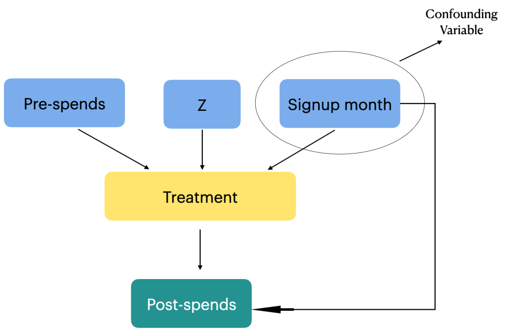
To estimate this effect, causal analysis aims to isolate the causal relationship between the membership program (treatment) and post-spends from other factors that may influence customer spending. These factors can include variables such as customers’ purchasing habits prior to signing up for the program, seasonality, and other unobserved factors. Addressing these potential confounding variables is crucial to obtain an accurate estimation of the causal effect of the membership program on post-spends. In our case we only have a single confounding factor which is the sign up month variable. We will be adjusting the effect of the confounding variable in our estimation.

By carefully accounting for confounding variables through methods like propensity score matching the causal analysis aims to provide reliable estimates of the treatment effect. These estimates help answer questions about the effectiveness of the membership program in influencing customer spending patterns and provide valuable insights for decision-making and program evaluation. Let us now look at the steps to estimate the effect using propensity score matching. The estimation would entail the following steps.

3.0 Steps in implementing causal estimation using PSM

Propensity Score Matching (PSM) unfolds in three pivotal steps. The journey begins with model fitting, often employing logistic regression to craft propensity scores that signify the likelihood of receiving treatment based on observed covariates. Following this, the matching phase seeks balance between treated and control groups, ensuring a fair and unbiased comparison. This involves pairing individuals with similar or identical propensity scores, akin to creating a controlled experiment from observational data. Finally, we estimate effects, scrutinizing the outcomes for the matched pairs to discern the causal impact of the treatment variable.

Model Fitting

Fit a model (e.g., logistic regression) to estimate the propensity scores. The model predicts the probability of receiving the treatment based on the observed covariates.

Matching:

Match each treated unit with one or more control units from the control group who have similar or close propensity scores.
The matching process aims to balance the covariates between the treatment and control groups, making them comparable.

Estimation:

Calculate the average treatment effect (ATE) or the average treatment effect on the treated (ATT) using the matched data.
The treatment effect is estimated by comparing the outcomes between the treated and matched control units.

We will explain each of these steps when we implement them. To implement these steps let us get back to the data frame we created in the previous blog and the separate out the data for the treatment, outcome and confounding variables

# Separating the treatment, outcome and confounding data
treatment_name = ['treatment']
outcome_name = ['post_spends']
common_cause_name = ['signup_month']
# Extracting the relevant data
treatment = df_i_signupmonth[treatment_name]
outcome = df_i_signupmonth[outcome_name]
common_causes = df_i_signupmonth[common_cause_name]

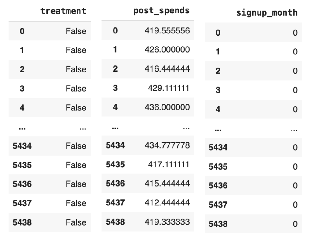
Figure 1: Snap shot of the treatment, outcome and common causes data

Let us now define the propensity score model, which we will fit with a logistic regression model.

from sklearn import linear_model
# Defining the propensity score model
propensity_score_model = linear_model.LogisticRegression()

Let us take a step back and understand the intuition behind defining a logistic regression model as our propensity score model.

The choice of a logistic regression model as the propensity score model in the context of the membership program is to estimate the probability of customers signing up for the program (treatment) based on their characteristics (common causes).

In causal analysis, the propensity score is defined as the conditional probability of receiving the treatment given the observed covariates. In the context of estimating the effect in causal analysis, the conditional probability helps address the issue of confounding variables. Confounding occurs when there are factors or variables that are associated with both the treatment and the outcome, and they distort the estimation of the causal effect. By conditioning on or adjusting for the common causes, we aim to create comparable groups of treated and control individuals with similar characteristics.

The propensity score model, such as logistic regression, estimates this conditional probability by modeling the relationship between the common causes and the probability of treatment.In the context of the membership program, by estimating the propensity score, we can adjust for the potential confounding variable (sign-up month) which may influence both the treatment assignment (being a member) and the outcome of interest (post spend). Confounding occurs when there are factors that are associated with both the treatment and the outcome, and failing to account for them can lead to biased estimates of the treatment effect.

Using the propensity score, we can match individuals who have similar probabilities of signing up for the program, effectively creating comparable groups in terms of their likelihood of being members. This matching process ensures that any differences in post spend between the treatment and control groups can be attributed primarily to the treatment itself, rather than the confounding effect of sign-up month. By isolating the causal effect of the membership program through propensity score matching, we can more accurately estimate how the program influences post spend for customers who have signed up.

Let us now estimate the propensity scores by fitting the model with the common causes and the treatment variable. Before we actually fit the model we have to reformat the data sets a bit.

# Reformatting the common causes and treatment variables
common_causes = pd.get_dummies(common_causes, drop_first=True)
treatment_reshaped = np.ravel(treatment)
# Fit the model using these variables
propensity_score_model.fit(common_causes, treatment_reshaped)
# Getting the propensity scores by predicting with the model
df_i_signupmonth['propensity_scores'] = propensity_score_model.predict_proba(common_causes)[:, 1]
df_i_signupmonth

Line 13 of code uses the pd.get_dummies() function to convert the common_causes variable into a one-hot encoded variable. This means that each of the categorical variables in the common_causes variable will be converted into a new binary variable. The drop_first=True argument tells the pd.get_dummies() function to drop the first level of the categorical variable. This is done because the first level is usually the reference level, and it does not provide any additional information.

Line 14 uses the np.ravel() function to convert the treatment variable into a 1D array. This is necessary because the propensity_score_model.fit() function expects a 1D array as the dependent variable.
Line 16 uses the propensity_score_model.fit() function to fit the model to the common_causes and treatment_reshaped variables. This function will estimate the coefficients of the model, which will be used to predict the propensity scores.

Line 18 uses the propensity_score_model.predict_proba() function to predict the propensity scores for each individual in the df_i_signupmonth DataFrame. The [:, 1] slice tells the propensity_score_model.predict_proba() function to return only the probability of receiving the treatment, which is the second column of the output array.

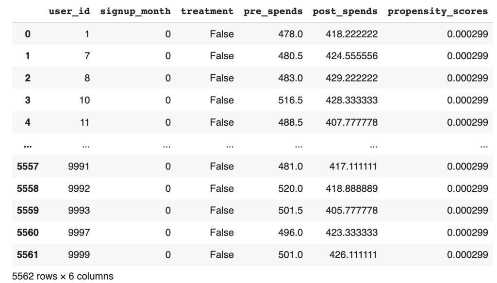
The new data frame with the prediction will be as below

Figure 2 : Dataframe with the propensity score predicted

From the data frame, the output propensity_scores represents the estimated probability of an individual signing up for the program given their observed characteristics (common causes). A higher propensity score indicates a higher probability of signing up for the membership program, and vice versa. By fitting the model and predicting the propensity scores, we obtain a quantitative measure of the likelihood of an individual being a member based on their observed characteristics.

These propensity scores are valuable in causal analysis because they allow for matching or stratification of individuals who have similar probabilities of treatment. By grouping individuals with similar propensity scores, we can create comparable treatment and control groups that are balanced in terms of their observed characteristics. This enables more accurate estimation of the causal effect by isolating the impact of the treatment (membership program) from other confounding factors. Let us now start the process

# Seperate the treated and control groups
treated = df_i_signupmonth.loc[df_i_signupmonth[treatment_name[0]] == 1]
control = df_i_signupmonth.loc[df_i_signupmonth[treatment_name[0]] == 0]

Figure 3: Treated and Control groups with predicted propensity score

From the separate data frames of treated and control, you can see the difference in the propensity scores. The treated group has much higher likelihood than the control group. Next we will find the neighbours for the treated and control groups respectively to find individuals of similar propensities.

In propensity score matching, the goal is to identify individuals in the control group who are similar to those in the treatment group based on their propensity scores. This is done to create a matched comparison group that closely resembles the treated group in terms of their likelihood of receiving the treatment.

# Import the required libraries
from sklearn.neighbors import NearestNeighbors
# Fit the nearest neighbour on the control group ( Have not signed up) propensity score
control_neighbors = NearestNeighbors(n_neighbors=1, algorithm="ball_tree").fit(control["propensity_scores"].values.reshape(-1, 1))
# Find the distance of the control group to each member of the treated group ( Individuals who signed up)
distances, indices = control_neighbors.kneighbors(treated["propensity_scores"].values.reshape(-1, 1))

Line 26 fits a nearest neighbors model on the control group’s propensity scores. This model will find the nearest neighbors of each individual in the control group, based on their propensity scores.

Line 28 then finds the distance of the control group to each member of the treated group. This is done by using the nearest neighbors model that was fit on the control group. The distance is calculated by finding the Euclidean distance between the propensity scores of the individuals in the control group and the propensity scores of the individuals in the treated group.

The reason why we fit the nearest neighbors model on the control group and then find its distance on the treated group is because we want to find the individuals in the control group who are most similar to the individuals in the treated group. By fitting the model on the control group, we can ensure that the distances are calculated based on the propensity scores of the control group.

This is important because we want to match individuals who are similar in terms of their propensity scores, so that we can control for confounding variables. If we were to fit the nearest neighbors model on the treated group, we would be matching individuals who are similar in terms of their propensity scores, but who may not be similar in terms of other confounding variables.

Having found the indices of the individuals in the control group, we will be able to calculate the average treatment effect of the treated ( ATT ).

ATT refers to the average causal effect of the treatment on the treated group. It estimates the average difference in the outcome variable between the treated group (those who received the treatment, in this case, signed up for the membership program) and their matched counterparts in the control group (those who did not receive the treatment).

The calculation of ATT involves comparing the outcomes of the treated group with their nearest neighbors in the control group, who have similar propensity scores. By matching individuals based on their propensity scores, we aim to create balanced comparison groups, where the only systematic difference between the treated and control group is the treatment itself. Let us look at how this is done

# Calculation of the ATT
att = 0
numtreatedunits = treated.shape[0]
for i in range(numtreatedunits):
  treated_outcome = treated.iloc[i][outcome_name].item()
  control_outcome = control.iloc[indices[i][0]][outcome_name].item()
  att += treated_outcome - control_outcome
att /= numtreatedunits
print('Average treatment effect of treated',att)

The provided code snippet calculates the ATT by computing the difference in outcomes between the treated group and their matched counterparts in the control group.

Line 32 iterates over each individual in the treated group and retrieves their outcome value. In lines 33-34, using the indices obtained from the nearest neighbor search, the corresponding control unit is identified and its outcome value is retrieved. The difference between the treated outcome and the matched control outcome is then computed and added to the ATT variable, as shown in line 35. This process is repeated for each treated individual. The resulting ATT value represents the average difference in outcomes between the treated and matched control group, providing an estimate of the causal effect of the membership program on the treated individuals. Finally the ATT is calculated by dividing by the number of treated individuals. We get a value of 93.45 for ATT.

An Average Treatment Effect of Treated (ATT) value of 93.45 suggests that, on average, individuals who received the treatment experienced an increase or improvement in the outcome variable by 93.45 units compared to if they had not received the treatment. In other words, the treatment is associated with a positive impact on the outcome.

ATT is relevant because it provides an estimate of the causal effect of the treatment specifically for those who received it. It helps us understand the impact of the membership program on the treated individuals’ outcomes, such as post-spending behavior, by accounting for potential confounding factors through propensity score matching.

Similarly let us calculate ATC which is the average treatment effect on the control group.

# Computing ATC
treated_neighbors = NearestNeighbors(n_neighbors=1, algorithm="ball_tree").fit(treated["propensity_scores"].values.reshape(-1, 1))
distances, indices = treated_neighbors.kneighbors(control["propensity_scores"].values.reshape(-1, 1))
# Calculating ATC from the neighbours of the control group
atc = 0
numcontrolunits = control.shape[0]
for i in range(numcontrolunits):
  control_outcome = control.iloc[i][outcome_name].item()
  treated_outcome = treated.iloc[indices[i][0]][outcome_name].item()
  atc += treated_outcome - control_outcome
atc /= numcontrolunits
print('Average treatment effect on control',atc)

We follow a similar process to find the ATC. Here the nearest neighbour is first fitted on the treatment group propensity score. Then the distance or similarity of each individual in the control group to a corresponding individual in the treated group is found out. After finding the neighbours the calculation of ATC is done similar to what we did for ATT.

Having found both ATT and ATC , we are in a position to calculate the estimate for Average Treatment Effect (ATE).

To calculate the ATE , we combine the ATT and ATC weighted by their respective proportion. The ATE represents the average causal effect of the treatment across both the treated and control groups.

The ATE can be calculated using the following formula:

ATE = (ATT * proportion of treated) + (ATC * proportion of control).

Let us now calculate the ATE

# Calculation of Average Treatment Effect
ate = (att * numtreatedunits + atc * numcontrolunits) / (numtreatedunits + numcontrolunits)
print('Average treatment effect',ate)

In the context of the membership program, the ATE holds significant relevance in understanding the impact of the program on customer spending behavior. Through causal analysis, we can estimate the ATE to assess the average causal effect of the program on post-spends. This involves considering factors such as the treatment group (customers who signed up for the program) and the control group (customers who did not sign up) while accounting for potential confounding variables.

By estimating the Average Treatment Effect on the Treated (ATT) and the Average Treatment Effect on the Control (ATC), we can gain valuable insights. A positive ATT would indicate that customers who signed up for the membership program have higher post-spends compared to those who did not sign up. Conversely, a negative ATT would suggest that signing up for the program leads to lower post-spends. The ATC provides a counterfactual comparison, indicating the outcomes that customers in the control group would have had if they had signed up for the program.

The ATE serves as a crucial measure to evaluate the overall impact of the membership program. A positive ATE would suggest that, on average, the program has a positive causal effect on customer post-spends. Conversely, a negative ATE would indicate a negative average causal effect. These findings help stakeholders assess the effectiveness of the program and make informed decisions regarding its implementation and continuation.

Implementing Causal analysis using do-why

In the last blog of the series we dealt with the processes involved in the causal identification namely, creating the causal graph, and then identifying different paths through which causal effect can flow like, back door paths, front door paths and instrumental variables. In our manual analysis of the causal graph we identified the presence of both back door and instrumental variables. Our causal graph did not have a front door variable. We did all the identification manually. We can implement all those processes in do-why also. Let us now see how the identification process can be done using do-why.

# Identification process
identified_estimand = model.identify_effect(proceed_when_unidentifiable=True)
print(identified_estimand)

The output generated from this process is as shown below. The output describes the various estimand’s or paths which are relevant. We can see that both the back door path and the instrumental variables have been identified.

Figure 4: Estimand for the causal analysis

Let us now understand above estimands and the different expressions used

Estimand 1 ( Back door )

Estimand Expression: This represents the causal effect of treatment on post_spends, adjusted for signup_month.

This expression is calculating the derivative of the expected value of post_spends with respect to the treatment variable treatment while controlling for the variable signup_month. In simpler terms, it’s looking at how the average post_spends changes when you change the treatment, considering the influence of signup_month to account for potential confounding.

Estimand Assumption 1 (Unconfoundedness): Assumes that there are no unobserved confounders (U) that simultaneously affect the treatment and outcome.The assumption of unconfoundedness is a fundamental requirement for making causal inferences using observational data. Let’s break down the statement:

This part of the assumption is saying that there are no unobserved confounders (U) that directly influence the treatment assignment. In other words, any factor that might influence both the treatment assignment and the outcome is already observed and included in the variables.

Similarly, there are no unobserved confounders that directly influence the outcome variable (post_spends).

Now, the main part of the assumption:

This is asserting that, conditional on treatment assignment (treatment), the month of signup (signup_month), and any observed variables (U), the distribution of post_spends is the same as if we condition only on treatment and signup_month. In simpler terms, it’s saying that, given what we know (treatment assignment, signup month, and any observed factors), the unobserved factors (represented by U) do not introduce bias or confounding.

Estimand 2 (Instrumental Variable):

Figure 5: Estimand expressions

This expression involves more complex calculus but, in essence, it’s estimating the causal effect of the treatment on post_spends using pre_spends and Z as instrumental variables. It’s essentially calculating the ratio of changes in post_spends with respect to changes in treatment, adjusted for changes in pre_spends and Z. The inverse of this is taken to estimate the causal effect.

Estimand Assumption 1: As-if-random

This assumption is related to the instrumental variable (Z). It’s asserting that if there are unobserved factors (U) that influence post_spends (as indicated by �⟶→ ⁣→U⟶→→), then those unobserved factors are not related to both the instrumental variable (Z) and the variables we’re controlling for (pre_spends). In other words, the instrumental variable is not correlated with the unobserved factors influencing the outcome, ensuring that it acts as a good instrument.

Estimand Assumption 2: Exclusion

This assumption is crucial for instrumental variables. It states that the instrumental variable (Z) and the variable we’re controlling for (pre_spends) do not have a direct effect on the outcome variable (post_spends). The idea is that the only influence these variables have on the outcome is through their impact on the treatment (treatment).

These assumptions ensure that the instrumental variable is a valid instrument for estimating the causal effect of the treatment on the outcome. The first part ensures that the instrumental variable is not correlated with unobserved factors affecting the outcome, and the second part ensures that the instrumental variable only affects the outcome through its impact on the treatment, not directly. Violations of these assumptions could lead to biased estimates.

Estimand 3 (Frontdoor):

No expression is provided in your example because DoWhy did not find a valid front door path.

The above are the processes which happen in the identification step. Once the identification process is complete we go on to the estimation method which we will see next.

# Estimation process
estimate = model.estimate_effect(identified_estimand,
                                 method_name="backdoor.propensity_score_matching",
                                target_units="ate")
print(estimate)

Let us look at the outputs and then unravel its content.

Figure 6: Estimand expressions

The above identified estimand expression aims to capture the causal effect of the treatment variable on post-spending while controlling for the covariate signup_month. The expression represents the derivative of the expected post-spending with respect to the treatment. The assumption of unconfoundedness ensures that there are no unobserved confounders affecting both the treatment assignment and post-spending.

The mean value of 112.27 for the Average Treatment Effect suggests that, on average, the treatment is associated with an increase of approximately 112.27 units in post-spending compared to the control group. Now in our manual method the estimate came to around 95. There is slight difference in both which can be attributed to the difference in random generation of data. However the direction in both the methods is the same.

Conclusion

In this dual-series exploration of causal analysis within the context of our loyalty membership program, we embarked on a comprehensive journey from the foundational principles to the advanced techniques that underpin causal inference. Our journey began with an elucidation of causal analysis, dissecting Average Treatment Effects (ATE), front door, back door, and instrumental variables. We navigated through the landscape of causal graphs, unraveling the relationships and dependencies that characterize our loyalty program dynamics. The second part of our exploration delved into causal identification and estimation, where we meticulously defined our causal questions and applied sophisticated methods to estimate causal effects. These blogs collectively provide a holistic understanding of the intricacies involved in discerning causation from correlation, equipping us with powerful tools to uncover the true impact of our loyalty membership program on customer behavior. As we conclude this series, we’ve not only enhanced our theoretical grasp of causal analysis but have also gained practical insights that can be applied across various domains, illuminating the path toward more informed decision-making in loyalty program management.

“Discover Data Science Wonders: Subscribe Now!”

Embark on a journey through the fascinating world of data science with our blog!

“Whether you’re a data enthusiast or just starting, we simplify complex concepts, turning data science into a delightful experience.”

Subscribe today to unravel the mysteries and gain insights.

But there’s more!

Join our YouTube channel for visual learning adventures.

Dive into data with us and make learning simple and fun.

Subscribe for your dose of data magic today! 🚀✨

Building Self Learning Recommendation system – V : Prototype Phase II : Self Learning Implementation

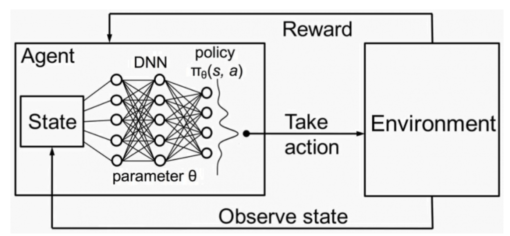
This is the fifth post of our series on building a self learning recommendation system using reinforcement learning. This post of the series builds on the previous post where we segmented customers using RFM analysis. This series consists of the following posts.

Recommendation system and reinforcement learning primer
Introduction to multi armed bandit problem
Self learning recommendation system as a K-armed bandit
Build the prototype of the self learning recommendation system : Part I
Build the prototype of the self learning recommendation system: Part II ( This post )
Productionising the self learning recommendation system: Part I – Customer Segmentation
Productionising the self learning recommendation system: Part II – Implementing self learning recommendation
Evaluating different deployment options for the self learning recommendation systems.

Introduction

In the last post we saw how to create customer segments from transaction data. In this post we will use the customer segments to create states of the customer. Before making the states let us make some assumptions based on the buying behaviour of customers.

Customers in the same segment have very similar buying behaviours
The second assumption we will make is that buying pattern of customers vary accross the months. Within each month we are assuming that the buying behaviour within the first 15 days is different from the buying behaviour in the next 15 days. Now these assumptions are made only to demonstrate how such assumptions will influence the creation of different states of the customer. One can still go much more granular with assumptions that the buying pattern changes every week in a month, i.e say the buying pattern within the first week will be differnt from that of the second week and so on. With each level of granularity the number of states required will increase. Ideally such decisions need to be made considering the business dynamics and based on real customer buying behaviours.
The next assumption we will be making is based on the days in a week. We make an assumption that buying behaviours of customers during different days of a week also varies.

Based on these assumptions, each state will have four tiers i.e

Customer segment >> month >> within first 15 days or not >> day of the week.

Let us now see how this assumption can be carried forward to create different states for our self learning recommendation system.

As a first step towards creation of states, we will create some more variables from the existing variables. We will be using the same dataframe we created till the segmentation phase, which we discussed in the last post.

# Feature engineering of the customer details data frame
# Get the date  as a seperate column
custDetails['Date'] = custDetails['Parse_date'].apply(lambda x: x.strftime("%d"))
# Converting date to float for easy comparison
custDetails['Date']  = custDetails['Date'] .astype('float64')
# Get the period of month column
custDetails['monthPeriod'] = custDetails['Date'].apply(lambda x: int(x > 15))

custDetails.head()

Let us closely look at the changes incorporated. In line 3, we are extracting the date of the month and then converting them into a float type in line 5. The purpose of taking the date is to find out which of these transactions have happened before 15th of the month and which after 15th. We extract those details in line 7, where we create a binary points ( 0 & 1) as to whether a date falls in the last 15 days or the first 15 days of the month. Now all data points required to create the state is in place. These individual data points will be combined together to form the state ( i.e. Segment-Month-Monthperiod-Day ). We will getinto nuances of state creation next.

Initialization of values

When we discussed about the K armed bandit in post 2, we saw the functions for generating the rewards and value. What we will do next is to initialize the reward function and the value function for the states.A widely used method for finding the value function and the reward function is to intialize those values to zero. However we already have data on each state and the product buying frequency for each of these states. We will aggregate the quantities of each product as per the state combination to create our initial value functions.

# Aggregate custDetails to get a distribution of rewards
rewardFull = custDetails.groupby(['Segment','Month','monthPeriod','Day','StockCode'])['Quantity'].agg('sum').reset_index()

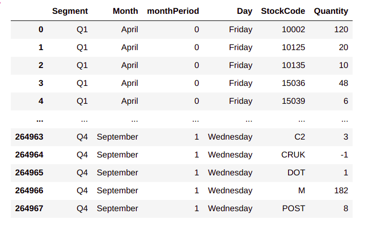
rewardFull

From the output, we can see the state wise distribution of products . For example for the state Q1_April_0_Friday we find that the 120 quantities of product ‘10002’ was bought and so on. So the consolidated data frame represents the propensity of buying of each product. We will make the propensity of buying the basis for the initial values of each product.

Now that we have consolidated the data, we will get into the task of creating our reward and value distribution. We will extract information relevant for each state and then load the data into different dictionaries for ease of use. We will kick off these processes by first extracting the unique values of each of the components of our states.

# Finding unique value for each of the segment 
segments = list(rewardFull.Segment.unique())
print('segments',segments)
months = list(rewardFull.Month.unique())
print('months',months)
monthPeriod = list(rewardFull.monthPeriod.unique())
print('monthPeriod',monthPeriod)
days = list(rewardFull.Day.unique())
print('days',days)

In lines 16-22, we take the unique values of each of the components of our state and then store them as list. We will use these lists to create our reward an value function dictionaries . First let us create dictionaries in which we are going to store the values.

# Defining some dictionaries for storing the values
countDic = {} # Dictionary to store the count of products
polDic = {} # Dictionary to store the value distribution
rewDic = {} # Dictionary to store the reward distribution
recoCount = {} # Dictionary to store the recommendation counts

Let us now implement the process of initializing the reward and value functions.

for seg in segments:
    for mon in months:
        for period in monthPeriod:
            for day in days:
                # Get the subset of the data
                subset1 = rewardFull[(rewardFull['Segment'] == seg) & (rewardFull['Month'] == mon) & (
                            rewardFull['monthPeriod'] == period) & (rewardFull['Day'] == day)]                
                # Check if the subset is valid
                if len(subset1) > 0:
                    # Iterate through each of the subset and get the products and its quantities
                    stateId = str(seg) + '_' + mon + '_' + str(period) + '_' + day
                    # Define a dictionary for the state ID
                    countDic[stateId] = {}                    
                    for i in range(len(subset1.StockCode)):
                        countDic[stateId][subset1.iloc[i]['StockCode']] = int(subset1.iloc[i]['Quantity'])

Thats an ugly looking loop. Let us unravel it. In lines 30-33, we implement iterative loops to go through each component of our state, starting from segment, month, month period and finally days. We then get the data which corresponds to each of the components of the state in line 35. In line 38 we do a check to see if there is any data pertaining to the state we are interested in. If there is valid data, then we first define an ID for the state, by combining all the components in line 40. In line 42, we define an inner dictionary for each element of the countDic, dictionary. The key of the countDic dictionary is the state Id we defined in line 40. In the inner dictionary we store each of the products as its key and the corresponding quantity values of the product as its values in line 44.

Let us look at the total number of states in the countDic

len(countDic)

You will notice that there are 572 states formed. Let us look at the data for some of the states.

stateId = 'Q4_September_1_Wednesday'
countDic[stateId]

From the output we can see how for each state, the products and its frequency of purchase is listed. This will form the basis of our reward distribution and also the value distribution. We will create that next

Consolidation of rewards and value distribution

from numpy.random import normal as GaussianDistribution

# Consolidate the rewards and value functions based on the quantities
for key in countDic.keys():    
    # First get the dictionary of products for a state
    prodCounts = countDic[key]
    polDic[key] = {}
    rewDic[key] = {}    
    # Update the policy values
    for pkey in prodCounts.keys():
        # Creating the value dictionary using a Gaussian process
        polDic[key][pkey] = GaussianDistribution(loc=prodCounts[pkey], scale=1, size=1)[0].round(2)
        # Creating a reward dictionary using a Gaussian process
        rewDic[key][pkey] = GaussianDistribution(loc=prodCounts[pkey], scale=1, size=1)[0].round(2)

In line 50, we iterate through each of the states in the countDic. Please note that the key of the dictionary is the state. In line 52, we store the products and its counts for a state, in another variable prodCounts. The prodCounts dictionary has the the product id as its key and the buying frequency as the value,. Lines 53 and 54, we create two more dictionaries for the value and reward dictionaries. In line 56 we loop through each product of the state and make it the key of the inner dictionaries of reward and value dictionaries. We generate a random number from a Gaussian distribution with the mean as the frequency of purchase for the product . We store the number generated from the Gaussian distribution as values for both rewards and value function dictionaries. At the end of the iterations, we get a distribution of rewards and value for each state and the products within each state. The distribution would be centred around the frequency of purchase of each of the product under the state.

Let us take a look at some sample values of both the dictionaries

polDic[stateId]

rewDic[stateId]

We have the necessary ingradients for building our selflearning recommendation engine. Let us now think about the actual process in an online recommendation system. In the actual process when a customer visits the ecommerce site, we first need to understand the state of that customer which will be the segment of the customer, the currrent month, which half of the month the customer is logging in and also the day when the customer is logging in. These are the information we would require to create the states.

For our purpose we will simulate the context of the customer using random sampling

Simulation of customer action

# Get the context of the customer. For the time being let us randomly select all the states
seg = sample(['Q1','Q2','Q3','Q4'],1)[0] # Sample the segment
mon = sample(['January','February','March','April','May','June','July','August','September','October','November','December'],1)[0] # Sample the month
monthPer = sample([0,1],1)[0] # sample the month period
day = sample(['Sunday','Monday','Tuesday','Wednesday','Thursday','Friday','Saturday'],1)[0] # Sample the day
# Get the state id by combining all these samples
stateId = str(seg) + '_' +  mon + '_' + str(monthPer) + '_' + day
print(stateId)

Lines 64-67, we sample each component of the state and then in line 68 we combine them to form the state id. We will be using the state id for the recommendation process. The recommendation process will have the following step.

Process 1 : Initialize dictionaries

A check is done to find if the value of reward dictionares which we earlier defined has the states which we sampled. If the state exists we take the value dictionary corresponding to the sampled state, if the state dosent exist, we initialise an empty dictionary corresponding to the state. Let us look at the function to do that.

def collfinder(dictionary,stateId):
    # dictionary ; This is the dictionary where we check if the state exists
    # stateId : StateId to be checked    
    if stateId in dictionary.keys():        
        mycol = {}
        mycol[stateId] = dictionary[stateId]
    else:
        # Initialise the state Id in the dictionary
        dictionary[stateId] = {}
        # Return the state specific collection
        mycol = {}
        mycol[stateId] = dictionary[stateId]
        
    return mycol[stateId],mycol,dictionary

In line 71, we define the function. The inputs are the dictionary the state id we want to verify. We first check if the state id exists in the dictionary in line 74. If it exists we create a new dictionary called mycol in line 75 and then load all the products and its count to mycol dictionary in line 76.

If the state dosent exist, we first initialise the state in line 79 and then repeat the same processes as of lines 75-76.

Let us now implement this step for the dictionaries which we have already created.

# Check for the policy Dictionary
mypolDic,mypol,polDic = collfinder(polDic,stateId)

Let us check the mypol dictionary.

mypol

We can see the policy dictionary for the state we defined. We will now repeat the process for the reward dictionary and the count dictionaries

# Check for the Reward Dictionary
myrewDic, staterew,rewDic = collfinder(rewDic,stateId)
# Check for the Count Dictionary
myCount,quantityDic,countDic = collfinder(countDic,stateId)

Both these dictionaries are similar to the policy dictionary above.

We also will be creating a similar dictionary for the recommended products, to keep count of all the products which are recommended. Since we havent created a recommendation dictionary, we will initialise that and create the state for the recommendation dictionary.

# Initializing the recommendation dictionary
recoCountdic = {}
# Check the recommendation count dictionary
myrecoDic,recoCount,recoCountdic = collfinder(recoCountdic,stateId)

We will now get into the second process which is the recommendation process

Process 2 : Recommendation process

We start the recommendation process based on the epsilon greedy method. Let us define the overall process for the recommendation system.

As mentioned earlier, one of our basic premise was that customers within the same segment have similar buying propensities. So the products which we need to recommend for a customer, will be picked from all the products bought by customers belonging to that segment. So the first task in the process is to get all the products relevant for the segment to which the customer belongs. We sort the products, in descending order, based on the frequency of product purchase.

Implementing the self learning recommendation system using epsilon greedy process

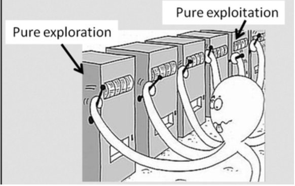
Next we start the epsion greedy process as learned in post 2, to select the top n products we want to recommend. To begin this process, we generate a random probability distribution value. If the random value is greater than the epsilon value, we pick the first product in the sorted list of products for the segment. Once a product is picked we remove it from the list of products from the segment to ensure that we dont pick it again. This process as we learned when we implemented K-armed bandit problem, is the exploitation phase.

The above was a case when the random probability number was greater than the epsilon value, now if the random probability number is less than the epsilon value, we get into the exploration phase. We randomly sample a product from the universe of products for the segment. Here again we restrict our exploration to the universe of products relevant for the segment. However one could design the exploration ourside the universe of the segment and maybe explore from the basket of all products for all customers.

We continue the exploitation and exploration process till we get the top n products we want. We will look at some of the functions which implements this process.

# Create a function to get a list of products for a certain segment
def segProduct(seg, nproducts,rewardFull):
    # Get the list of unique products for each segment
    seg_products = list(rewardFull[rewardFull['Segment'] == seg]['StockCode'].unique())
    seg_products = sample(seg_products, nproducts)
    return seg_products

# This is the function to get the top n products based on value
def sortlist(nproducts, stateId,seg,mypol):
    # Get the top products based on the values and sort them from product with largest value to least
    topProducts = sorted(mypol[stateId].keys(), key=lambda kv: mypol[stateId][kv])[-nproducts:][::-1]
    # If the topProducts is less than the required number of products nproducts, sample the delta
    while len(topProducts) < nproducts:
        print("[INFO] top products less than required number of products")
        segProducts = segProduct(seg,(nproducts - len(topProducts)))
        newList = topProducts + segProducts
        # Finding unique products
        topProducts = list(OrderedDict.fromkeys(newList))
    return topProducts

# This is the function to create the number of products based on exploration and exploitation
def sampProduct(seg, nproducts, stateId, epsilon,mypol):
    # Initialise an empty list for storing the recommended products
    seg_products = []
    # Get the list of unique products for each segment
    Segment_products = list(rewardFull[rewardFull['Segment'] == seg]['StockCode'].unique())
    # Get the list of top n products based on value
    topProducts = sortlist(nproducts, stateId,seg,mypol)
    # Start a loop to get the required number of products
    while len(seg_products) < nproducts:
        # First find a probability
        probability = np.random.rand()
        if probability >= epsilon:            
            # The top product would be first product in the list
            prod = topProducts[0]
            # Append the selected product to the list
            seg_products.append(prod)
            # Remove the top product once appended
            topProducts.pop(0)
            # Ensure that seg_products is unique
            seg_products = list(OrderedDict.fromkeys(seg_products))
        else:
            # If the probability is less than epsilon value randomly sample one product
            prod = sample(Segment_products, 1)[0]
            seg_products.append(prod)
            # Ensure that seg_products is unique
            seg_products = list(OrderedDict.fromkeys(seg_products))
    return seg_products

In line 117 we define the function to get the recommended products. The input parameters for the function are the segment, number of products we want to recommend, state id,epsilon value and the policy dictionary . We initialise a list to store the recommended products in line 119 and then extract all the products relevant for the segment in line 121. We then sort the segment products according to frequency of the products. We use the function ‘sortlist‘ in line 104 for this purpose. We sort the value dictionary according to the frequency and then select the top n products in the descending order in line 106. Now if the number of products in the dictionary is less than the number of products we want to be recommended, we randomly select the remaining products from the list of products for the segment. Lines 99-100 in the function ‘segproducts‘ is where we take the list of unique products for the segment and then randomly sample the required number of products and return it in line 110. In line 111 the additional products along with the top products is joined together. The new list of top products are sorted as per the order in which the products were added in line 112 and returned to the calling function in line 123.

Lines 125-142 implements the epsilon greedy process for product recommendation. This is a loop which continues till we get the required number of products for recommending. In line 127 a random probability score is generated and is verified whether it is greater than the epsilon value in line 128. If the random probability score is greater than epsilon value, we extract the topmost product from the list of products in line 130 and then append it to the recommendation candidate product list in line 132. After extraction of the top product, it is removed from the list in line 134. The list is sorted according to the order in which products are added in line 136. This loop continues till we get the required number of products for recommendation.

Lines 137-142 is the loop when the random score is less than the epsilon value i.e exploration stage. In this stage we randomly sample products from the list of products appealing to the segment and append it to the list of recommendation candidates. The final list of candiate products to be recommended is returned in line 143.

Process 3 : Updation of all relevant dictionaries

In the last section we saw the process of selecting the products for recommendation. The next process we will cover is how the products recommended are updated in the relevant dictionaries like quantity dictionary, value dictionary, reward dictionary and recommendation dictionary. Again we will use a function to update the dictionaries. The first function we will see is the one used to update sampled products.

def dicUpdater(prodList, stateId,countDic,recoCountdic,polDic,rewDic):
    # Loop through each of the products
    for prod in prodList:        
        # Check if the product is in the dictionary
        if prod in list(countDic[stateId].keys()):
            # Update the count by 1
            countDic[stateId][prod] += 1            
        else:
            countDic[stateId][prod] = 1            
        if prod in list(recoCountdic[stateId].keys()):            
            # Update the recommended products with 1
            recoCountdic[stateId][prod] += 1           
        else:
            # Initialise the recommended products as 1
            recoCountdic[stateId][prod] = 1            
        if prod not in list(polDic[stateId].keys()):
            # Initialise the value as 0
            polDic[stateId][prod] = 0            
        if prod not in list(rewDic[stateId].keys()):            
            # Initialise the reward dictionary as 0
            rewDic[stateId][prod] = GaussianDistribution(loc=0, scale=1, size=1)[0].round(2)     
            
    # Return all the dictionaries after update
    return countDic,recoCountdic,polDic,rewDic

The inputs for the function are the recommended products ,prodList , stateID, count dictionary, recommendation dictionary, value dictionary and reward dictionary as shown in line 144.

A inner loop is executed in lines 146-166, to go through each product in the product list. In line 148 a check is made to find out if the product is in the count dictionary. This entails, understanding if the product was ever bought under that state. If the product was ever bought before, the count is updated by 1. However if the product was not bought earlier, then the dictionary for that product under that state is initialised as 1 in line 152.

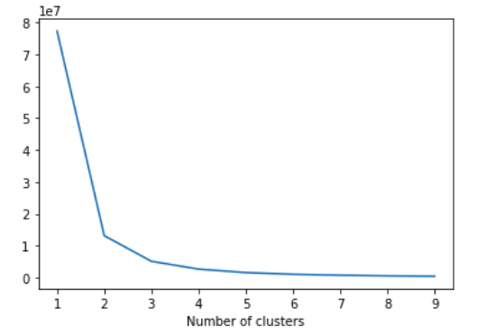
The next step is for updating the recommendation count for the same product. The same logic as above applies. If the product was recommended before, for that state, the number is updated by 1 if not the number is initialised to 1 in lines 153-158.

The next task is to verify if there is a value distribution for this product for the specific state as in lines 159-161. If the value distribution does not exist, it is initialised to zero. However we dont do any updation to the value distribution here. The updation to value distribution happens later on. We will come to that in a moment

The last check is to verify if the product exists in the reward dictionary for that state in lines 162-164. If it dosent exist then it is initialised with a gaussian distribution. Again we dont do any updation for reward as this is done later on.

Now that we have seen the function for updating the dictionaries, we will get into a function which initializes dictionaries. This process is required, if a particular state has never been seen for any of the dictionaries. Let us get to that function

def dicAdder(prodList, stateId,countDic,recoCountdic,polDic,rewDic):
    countDic[stateId] = {}
    polDic[stateId] = {}
    recoCountdic[stateId] = {}
    rewDic[stateId] = {}    
    # Loop through the product list
    for prod in prodList:
        # Initialise the count as 1
        countDic[stateId][prod] = 1
        # Initialise the value as 0
        polDic[stateId][prod] = 0
        # Initialise the recommended products as 1
        recoCountdic[stateId][prod] = 1
        # Initialise the reward dictionary as 0
        rewDic[stateId][prod] = GaussianDistribution(loc=0, scale=1, size=1)[0].round(2)
    # Return all the dictionaries after update
    return countDic,recoCountdic,polDic,rewDic

The inputs to this function as seen in line 168 are the same as what we saw in the update function. In lines 169-172, we initialise the innner dictionaries for the current state. Lines 174-182, all the inner dictionaries are initialised for the respective products. The count and recommendation dictionaries are initialised by 1 and the value dictionary is intialised as 0. The reward dictionary is initialised using a gaussian distribution. Finally the updated dictionaries are returned in line 184.

Next we start the recommendation process using all the functions we have defined so far.

nProducts = 10
epsilon=0.1

# Get the list of recommended products and update the dictionaries.The process is executed for a scenario when the context exists and does not exist
if len(mypolDic) > 0:    
    print("The context exists")
    # Implement the sampling of products based on exploration and exploitation
    seg_products = sampProduct(seg, nProducts , stateId, epsilon,mypol)
    # Update the dictionaries of values and rewards
    countDic,recoCountdic,polDic,rewDic = dicUpdater(seg_products, stateId,countDic,recoCountdic,polDic,rewDic)
else:
    print("The context dosent exist")
    # Get the list of relavant products
    seg_products = segProduct(seg, nProducts)
    # Add products to the value dictionary and rewards dictionary
    countDic,recoCountdic,polDic,rewDic = dicAdder(seg_products, stateId,countDic,recoCountdic,polDic,rewDic)

We define the number of products and epsilon values in lines 185-186. In line 189 we check if the state exists which would mean that there would be some products in the dictionary. If the state exists, then we get the list of recommended products using the ‘sampProducts‘ function we saw earlier in line 192. After getting the list of products we update all the dictionaries in line 194.

If the state dosent exist, then products are randomly sampled using the ‘segProduct‘ function in line 198. As before we update the dictionaries in line 200.

Process 4 : Customer Action

So far we have implemented the recommendation process. In real world application, the products we generated are displayed as recommendations to the customer. Based on the recommendations received, the customer carries out different actions as below.

Customer could buy one or more of the recommended products
Customer could browse through the recommended products
Customer could ignore all the recommendations.

Based on the customer actions, we need to give feed back to the online learning system as to how good the recommendations were. Obviously the first scenario is the most desired one, the second one indicates some level of interest and the last one is the undesirable effect. From an self learning perspective we need to reinforce the desirable behaviours and discourage undesirable behavrious by devising proper rewards systems.

Just like we simulated customer states, we will create some functions to simulate customer actions. We define probability distribution to simulate customers propensity for buying a product or clicking a product. Based on the probability distribution we get how many products get bought or how many get clicked. Based on these numbers we sample products from our recommended list as to how many of them are going to be bought or how many would be clicked. Please note that these processes are only required as we are not implementing on a real system. When we are implementing this process in a real system, we get all these feedbacks from the the choices made by the customer.

def custAction(segproducts):
    print('[INFO] getting the customer action')
    # Sample a value to get how many products will be clicked    
    click_number = np.random.choice(np.arange(0, 10), p=[0.50,0.35,0.10, 0.025, 0.015,0.0055, 0.002,0.00125,0.00124,0.00001])
    # Sample products which will be clicked based on click number
    click_list = sample(segproducts,click_number)

    # Sample for buy values    
    buy_number = np.random.choice(np.arange(0, 10), p=[0.70,0.15,0.10, 0.025, 0.015,0.0055, 0.002,0.00125,0.00124,0.00001])
    # Sample products which will be bought based on buy number
    buy_list = sample(segproducts,buy_number)

    return click_list,buy_list

The input to the function is the recommended products as seen from line 201. We then simulate the number of products the customer is going to click using a probability distribution shown in line 204. From the probability distribution we can see there is 50% of chance for not clicking any product, 35% chance to click one product and so on. Once we get the number of products which are likely to be clicked, we sample that many products from the recommended product list. We do a similar process for products that are likely to be bought in lines 209-211. Finally we return the list of products that will be clicked and bought. Please note that there is high likelihood that the returned lists will be empty as the probability distributions are skewed heavily towards that possiblity. Let us implement that function and see what we get.

click_list,buy_list = custAction(seg_products)
print(click_list)
print(buy_list)

So from the simulation, we can see that the customer browsed one product however did not buy any of the products. Please note that you might get a very different simulation when you try as this is a random sampling of products.

Now that we have got the customer action, our next step is to get rewards based on the customer actions. As reward let us define that we will give 5 points if the customer has bought a product and a reward of 1 if the customer has clicked the product and -2 reward if the customer has done neither of these.We will define some functions to update the value dictionaries based on the rewards.

def getReward(loc):
    rew = GaussianDistribution(loc=loc, scale=1, size=1)[0].round(2)
    return rew

def saPolicy(rew, stateId, prod,polDic,recoCountdic):
    # This function gets the relavant algorithm for the policy update
    # Get the current value of the state    
    vcur = polDic[stateId][prod]    
    # Get the counts of the current product
    n = recoCountdic[stateId][prod]    
    # Calculate the new value
    Incvcur = (1 / n) * (rew - vcur)    
    return Incvcur

def valueUpdater(seg_products, loc,custList,stateId,rewDic,polDic,recoCountdic, remove=True):
    for prod in custList:       
        # Get the reward for the bought product. The reward will be centered around the defined reward for each action
        rew = getReward(loc)        
        # Update the reward in the reward dictionary
        rewDic[stateId][prod] += rew        
        # Update the policy based on the reward
        Incvcur = saPolicy(rew, stateId, prod,polDic,recoCountdic)        
        polDic[stateId][prod] += Incvcur        
        # Remove the bought product from the product list
        if remove:
            seg_products.remove(prod)
    return seg_products,rewDic,polDic,recoCountdic

The main function is in line 231, whose inputs are the following,

seg_products : segment products we earlier derived

loc : reward for action ( i.e 5 for buy, 1 for browse and -2 for ignoring)

custList : The list of products which are clicked or bought by the customer

stateId : The state ID

rewDic,polDic,recoCountdic : Reward dictionary, value dictionary and recommendation count dictionary for updates

An iterative loop is initiated from line 232 to iterate through all the products in the corresponding list ( buy or click list). First we get the corresponding reward for the action in line 234. This line calls a function defined in line 217, which returns the reward from a Gaussian distribution centred at the reward location ( 5, 1 or -2). Once we get the reward we update the reward dictionary in line 236 with the new reward.

In line 238 we call the function ‘saPolicy‘ for getting the new value for the action. The function ‘saPolicy‘ defined in line 221, takes the reward, state Id , product and dictionaries as input and output the new values for updating the policy dictionary.

In line 224, we get the current value for the state and the product and in line 226 we get the number of times that product was ever selected. The new value is calculated in line 228 through the simple averaging method we dealt with in our post on K armed bandits. The new value is then returned to the calling function and then incremented with the existing value in lines 238-239. To avoid re-recommending the current product for the customer we do a check in line 241 and then remove it from the segment products in line 242. The updated list of segment products along with the updated dictionaries are then returned in line 243.

Let us now look at the implementation of these functions next.

if len(buy_list) > 0:
    seg_products,rewDic,polDic,recoCountdic = valueUpdater(seg_products, 5, buy_list,stateId,rewDic,polDic,recoCountdic)
    # Repeat the same process for customer click
if len(click_list) > 0:
    seg_products,rewDic,polDic,recoCountdic = valueUpdater(seg_products, 1, click_list,stateId,rewDic,polDic,recoCountdic)
    # For those products not clicked or bought, give a penalty
if len(seg_products) > 0:
    custList = seg_products.copy()
    seg_products,rewDic,polDic,recoCountdic = valueUpdater(seg_products, -2, custList,stateId ,rewDic,polDic,recoCountdic, False)

In lines 245,248 and 252 we update the values for the buy list, click list and the ignored products respectively. In the process all the dictionaries also get updated.

That takes us to the end of all the processes for the self learning system. When implementing these processes as system, we have to keep implementing these processes one by one. Let us summarise all the processes which needs to be repeated to build this self learning recommendation system.

Identify the customer context by simulating the states. In a real life system we dont have to simulate this information as this will be available when a customer logs in
Initialise the dictionaries for the state id we generated
Get the list of products to be recommended based on the state id
Update the dictionaries based on the list of products which were recommended
Simulate customer actions on the recommended products. Again in real systems we done simulate customer actions as it will be captured online.
Update the value dictionary and reward dictionary based on customer actions.

All these 6 steps will have to be repeated for each customer instance. Once this cycle runs for some continuous steps, we will get the value dictionaries updated and dynamically aligned to individual customer segments.

What next ?

In this post we built our self learning recommendation system using Jupyter notebooks. Next we will productionise these processes using python scripts. When we productionise these processes, we will also use Mongo DB database to store and retrieve data. We will start the productionising phase in the next post.

Please subscribe to this blog post to get notifications when the next post is published.

You can also subscribe to our Youtube channel for all the videos related to this series.

The complete code base for the series is in the Bayesian Quest Git hub repository

Do you want to Climb the Machine Learning Knowledge Pyramid ?

Knowledge acquisition is such a liberating experience. The more you invest in your knowledge enhacement, the more empowered you become. The best way to acquire knowledge is by practical application or learn by doing. If you are inspired by the prospect of being empowerd by practical knowledge in Machine learning, subscribe to our Youtube channel

I would also recommend two books I have co-authored. The first one is specialised in d eep learning with practical hands on exercises and interactive video and audio aids for learning

This book is accessible using the following links

The Deep Learning Workshop on Amazon

The Deep Learning Workshop on Packt

The second book equips you with practical machine learning skill sets. The pedagogy is through practical interactive exercises and activities.

This book can be accessed using the following links

The Data Science Workshop on Amazon

The Data Science Workshop on Packt

Enjoy your learning experience and be empowered !!!!

Building Self Learning Recommendation system – IV : Prototype Phase I: Segmenting the customers.

This is the fourth post of our series on building a self learning recommendation system using reinforcement learning. In the coming posts of the series we will expand on our understanding of the reinforcement learning problem and build an application for recommending products. These are the different posts of the series where we will progressively build our recommendation system.

Recommendation system and reinforcement learning primer
Introduction to multi armed bandit problem
Self learning recommendation system as a K-armed bandit
Build the prototype of the self learning recommendation system: Part I ( This post )
Build the prototype of the self learning recommendation system: Part II
Productionising the self learning recommendation system: Part I – Customer Segmentation
Productionising the self learning recommendation system: Part II – Implementing self learning recommendation
Evaluating different deployment options for the self learning recommendation systems.

Introduction

In the last post of the series we formulated the idea on how we can build the self learning recommendation system as a K armed bandit. In this post we will go ahead and start building the prototype of our self learning system based on the idea we developed. We will be using Jupyter notebook to build our prototype. Let us dive in

Processes for building our self learning recommendation system

Let us take a birds eye view of the recommendation system we are going to build. We will implement the following processes

Cleaning of the data set
Segment the customers using RFM segmentation
Creation of states for contextual recommendation
Creation of reward and value distributions
Implement the self learning process using simple averaging method
Simulate customer actions to initiate self learning for recommendations

The first two processes will be implemented in this post and the remaining processes will be covered in the next post.

Cleaning the data set

The data set which we would be using for this exercise would be the online retail data set. Let us load the data set in our system and get familiar with the data. First let us import all the necessary library files

from pickle import load
from pickle import dump
import numpy as np
import pandas as pd
from dateutil.parser import parse
import os
from collections import Counter
import operator
from random import sample

We will now define a simple function to load the data using pandas.

def dataLoader(orderPath):
    # THis is the method to load data from the input files    
    orders = pd.read_csv(orderPath,encoding = "ISO-8859-1")
    return orders

The above function reads the csv file and returns the data frame. Let us use this function to load the data and view the head of the data

# Please define your specific path where the data set is loaded
filename = "OnlineRetail.csv"
# Let us load the customer Details
custDetails = dataLoader(filename)
custDetails.head()

Further in the exercise we have to work a lot with the dates and therefore we need to extract relevant details from the date column like the day, weekday, month, year etc. We will do that with the date parser library. Let us now parse all the date related column and create new columns storing the new details we extract after parsing the dates.

#Parsing  the date
custDetails['Parse_date'] = custDetails["InvoiceDate"].apply(lambda x: parse(x))
# Parsing the weekdaty
custDetails['Weekday'] = custDetails['Parse_date'].apply(lambda x: x.weekday())
# Parsing the Day
custDetails['Day'] = custDetails['Parse_date'].apply(lambda x: x.strftime("%A"))
# Parsing the Month
custDetails['Month'] = custDetails['Parse_date'].apply(lambda x: x.strftime("%B"))
# Extracting the year
custDetails['Year'] = custDetails['Parse_date'].apply(lambda x: x.strftime("%Y"))
# Combining year and month together as one feature
custDetails['year_month'] = custDetails['Year'] + "_" +custDetails['Month']

custDetails.head()

Figure 2 : Data frame after date parsing

As seen from line 22 we have used the lambda() function to first parse the ‘date’ column. The parsed date is stored in a new column called ‘Parse_date’. After parsing the dates first, we carry out different operations, again using the lambda() function on the parsed date. The different operations we carry out are

Extract weekday and store it in a new column called ‘Weekday’ : line 24
Extract the day of the week and store it in the column ‘Day’ : line 26
Extract the month and store in the column ‘Month’ : line 28
Extract year and store in the column ‘Year’ : line 30

Finally, in line 32 we combine the year and month to form a new column called ‘year_month’. This is done to enable easy filtering of data based on the combination of a year and month.

We will also create a column which gives you the gross value of each puchase. Gross value can be calculated by multiplying the quantity with unit price.

# Creating gross value column
custDetails['grossValue'] = custDetails["Quantity"] * custDetails["UnitPrice"]
custDetails.head()

The reason we are calculating the gross value is to use it for segmentation of customers which will be dealt with in the next section. This takes us to the end of the initial preparation of the data set. Next we start creating customer segments.

Creating Customer Segments

In the last post, where we formulated the problem statement, we identified that customer segment could be one of the important components of the states. In addition to the customer segment,the other components are day of purchase and period of the month. So our next endeavour is to prepare data to create the different states we require. We will start with defining the customer segment.

There are different approaches to creating customer segments. In this post we will use the RFM analysis to create customer segments. Let us get going with creation of customer segments from our data set. We will continue on the same notebook we were using so far.

import lifetimes

In line 39,We import the lifetimes package to create the RFM data from our transactional dataset. Next we will use the package to convert the transaction data to the specific format.

# Converting data to RFM format
RfmAgeTrain = lifetimes.utils.summary_data_from_transaction_data(custDetails, 'CustomerID', 'Parse_date', 'grossValue')
RfmAgeTrain

The process for getting the frequency, recency and monetary value is very simple using the life time package as shown in line 42 . From the output we can see the RFM data frame formed with each customer ID as individual row. For each of the customer, the frequency and recency in days is represented along with the average monetary value for the customer. We will be using these values for creating clusters of customer segments.

Before we work further, let us clean the data frame a bit by resetting the index values as shown in line 44

RfmAgeTrain = RfmAgeTrain.reset_index()
RfmAgeTrain

What we will now do is to use recency, frequency and monetary values seperately to create clusters. We will use the K-means clustering technique to find the number of clusters required. Many parts of the code used for clustering is taken from the following post on customer segmentation.

In lines 46-47 we import the Kmeans clustering method and matplotlib library.

from sklearn.cluster import KMeans
import matplotlib.pyplot as plt

For the purpose of getting the recency matrix let us take a subset of the data frame with only customer ID and recency value as shown in lines 48-49

user_recency = RfmAgeTrain[['CustomerID','recency']]
user_recency.head()

In any clustering problem,as you might know, one of the critical tasks is to determine the number of clusters which in the Kmeans algorithm is a parameter. We will use the well known elbow method to find the optimum number of clusters.

# Initialize a dictionary to store sum of squared error
sse = {}
recency = user_recency[['recency']]

# Loop through different cluster combinations
for k in range(1,10):
    # Fit the Kmeans model using the iterated cluster value
    kmeans = KMeans(n_clusters=k,max_iter=2000).fit(recency)
    # Store the cluster against the sum of squared error for each cluster formation   
    sse[k] = kmeans.inertia_
    
# Plotting all the clusters
plt.figure()
plt.plot(list(sse.keys()),list(sse.values()))
plt.xlabel("Number of clusters")
plt.show()

In line 51, we initialise a dictionary to store the sum of square error for each k-means cluster and then subset the data frame ‘recency’ with only the recency values in line 52.

From line 55, we start a loop to itrate through different cluster values. For each cluster value, we fit the k-means model in line 57. We also store the sum of squared error in line 59 for each of the cluster in the dictionary we initialized.

Lines 62-65, we visualise the number of clusters against the sum of squared error, which gives and indication of the right k value to choose.

From the plot we can see that 2,3 and 4 cluster values are where the elbow tapers and one of these values can be taken as the cluster value.Let us choose 4 clusters for our purpose and then refit the data.

# let us take four clusters 
kmeans = KMeans(n_clusters=4)
# Fit the model on the recency data
kmeans.fit(user_recency[['recency']])
# Predict the clusters for each of the customer
user_recency['RecencyCluster'] = kmeans.predict(user_recency[['recency']])
user_recency

In line 67, we instantiate the KMeans class using 4 clusters. We then use the fit method on the recency values in line 69. Once the model is fit, we predict the cluster for each customer in line 71.

From the output we can see that the recency cluster is predicted against each customer ID. We will clean up this data frame a bit, by resetting the index.

user_recency.sort_values(by='recency',ascending=False).reset_index(drop=True)

From the output we can see that the data is ordered according to the clusters. Let us also look at how the clusters are mapped vis a vis the actual recency value. For doing this, we will group the data with respect to each cluster and then find the mean of the recency value, as in line 74.

user_recency.groupby('RecencyCluster')['recency'].mean().reset_index()

From the output we see the mean value of recency for each cluster. We can clearly see that there is a demarcation of the mean values with the value of the cluster. However, the mean values are not mapped in a logical (increasing or decreasing) order of the clusters. From the output we can see that cluster 3 is mapped to the smallest recency value ( 7.72). The next smallest value (115.85) is mapped to cluster 0 and so on. So there is not specific ordering to the custer and the mean value mapping. This might be a problem when we combine all the clusters for recency, frequency and monetary together to derive a combined score. So it is necessary to sort it in an ordered fashion. We will use a custom function to get the order right. Let us see the function.

# Function for ordering cluster numbers

def order_cluster(cluster_field_name,target_field_name,data,ascending):    
    # Group the data on the clusters and summarise the target field(recency/frequency/monetary) based on the mean value
    data_new = data.groupby(cluster_field_name)[target_field_name].mean().reset_index()
    # Sort the data based on the values of the target field
    data_new = data_new.sort_values(by=target_field_name,ascending=ascending).reset_index(drop=True)
    # Create a new column called index for storing the sorted index values
    data_new['index'] = data_new.index
    # Merge the summarised data onto the original data set so that the index is mapped to the cluster
    data_final = pd.merge(data,data_new[[cluster_field_name,'index']],on=cluster_field_name)
    # From the final data drop the cluster name as the index is the new cluster
    data_final = data_final.drop([cluster_field_name],axis=1)
    # Rename the index column to cluster name
    data_final = data_final.rename(columns={'index':cluster_field_name})
    return data_final

In line 77, we define the function and its inputs. Let us look at the inputs to the function

cluster_field_name : This is the field name we give to the cluster in the data set like “RecencyCluster”.

target_field_name : This is the field pertaining to our target values like ‘recency’ , ‘frequency’ and ,’monetary_values’.

data : This is the data frame containing the cluster information and target values, for eg ( user_recency)

ascending : This is a flag indicating whether the data has to be sorted in ascending order or not

Line 79, we group the data based on the cluster and summarise the data under each group to get the mean of the target variable. The idea is to sort the data frame based on the mean values in ascending order which is done in line 81. Once the data is sorted in ascending order, we form a new feature with the data frame index as its values, in line 83. Now the index values will act as sorted cluster values and we will get a mapping between the existing cluster values and the new cluster values which are sorted. In line 85, we merge the summarised data frame with the original data frame so that the new cluster values are mapped to all the values in the data frame. Once the new sorted cluster labels are mapped to the original data frame, the old cluster labels are dropped in line 87 and the column renamed in line 89

Now that we have defined the function, let us implement it and sort the data frame in a logical order in line 91.

user_recency = order_cluster('RecencyCluster','recency',user_recency,False)

Next we will summarise the new sorted data frame and check if the clusters and mapped in a logical order.

user_recency.groupby('RecencyCluster')['recency'].mean().reset_index()

From the above output we can see that the cluster numbers are mapped in a logical order of decreasing recency.
We now need to repeat the process for frequency and monetary values. For convenience we will wrap all these processes in a new function.

def clusterSorter(target_field_name,ascending):    
    # Make the subset data frame using the required feature
    user_variable = RfmAgeTrain[['CustomerID',target_field_name]]
    # let us take four clusters indicating 4 quadrants
    kmeans = KMeans(n_clusters=4)
    kmeans.fit(user_variable[[target_field_name]])
    # Create the cluster field name from the target field name
    cluster_field_name = target_field_name + 'Cluster'
    # Create the clusters
    user_variable[cluster_field_name] = kmeans.predict(user_variable[[target_field_name]])
    # Sort and reset index
    user_variable.sort_values(by=target_field_name,ascending=ascending).reset_index(drop=True)
    # Sort the data frame according to cluster values
    user_variable = order_cluster(cluster_field_name,target_field_name,user_variable,ascending)
    return user_variable

Let us now implement this function to get the clusters for frequency and monetary values.

# Implementing for user frequency
user_freqency = clusterSorter('frequency',True)
user_freqency.groupby('frequencyCluster')['frequency'].mean().reset_index()

# Implementing for monetary values
user_monetary = clusterSorter('monetary_value',True)
user_monetary.groupby('monetary_valueCluster')['monetary_value'].mean().reset_index()

Let us now sit back and look at the three results which we got and try to analyse the results. For recency, we implemented the process using ‘ascending’ value as ‘False’ and the other two with ascending value as ‘True’. Why do you think we did it this way ?

To answer let us look these three variables from the perspective of the desirable behaviour from a customer. We would want customers who are very recent, are very frequent and spent lot of money. So from a recency perspective lesser days is a good behaviour as this indicate very recent customers. The reverse is true for frequency and monetary where the more of those values is the desirable behaviour. This is why we used 'ascending = false' in the recency variable as the clusters would be sorted with the less frequent ( more days) for cluster ‘0’ and the mean days comes down when we go to cluster 3. So in effect we are making cluster 3 as the group of most desirable customers. The reverse applies to frequency and monetary value where we gave 'ascending = True' to make custer 3 as the group of most desirable customers.

Now that we have obtained the clusters for each of the variables seperately, its time to combine them into one data frame and then get a consolidated score which will become the segments we want.

Let us first combine each of the individual dataframes we created with the original data frame

# Merging the individual data frames with the main data frame
RfmAgeTrain = pd.merge(RfmAgeTrain,user_monetary[["CustomerID",'monetary_valueCluster']],on='CustomerID')
RfmAgeTrain = pd.merge(RfmAgeTrain,user_freqency[["CustomerID",'frequencyCluster']],on='CustomerID')
RfmAgeTrain = pd.merge(RfmAgeTrain,user_recency[["CustomerID",'RecencyCluster']],on='CustomerID')
RfmAgeTrain.head()

In lines 115-117, we combine the individual dataframes to our main dataframe. We combine them on the ‘CustomerID’ field. After combining we have a consolidated data frame with each individual cluster label mapped to each customer id as shown below

Let us now add the individual cluster labels to get a combined cluster score.

# Calculate the overall score
RfmAgeTrain['OverallScore'] = RfmAgeTrain['RecencyCluster'] + RfmAgeTrain['frequencyCluster'] + RfmAgeTrain['monetary_valueCluster']
RfmAgeTrain

Let us group the data based on the ‘OverallScore’ and find the mean values of each of our variables , recency, frequency and monetary.

RfmAgeTrain.groupby('OverallScore')['frequency','recency','monetary_value'].mean().reset_index()

From the output we can see how the distributions of the new clusters are. From the values we can see that there is some level of logical demarcation according to the cluster labels. The higher cluster labels ( 4,5 & 6) have high monetary values, high frequency levels and also mid level recency levels. The first two clusters ( 0 & 1) have lower monetary values, high recency and low levels of frequency. Another stand out cluster is cluster 3, which has the lowest monetary value, lowest frequency and the lowest recency. We can very well go with these six clusters or we can combine clusters who demonstrate similar trends/behaviours. However this assessment needs to be taken based on the number of customers we have under each of these new clusters. Let us get those numbers first.

RfmAgeTrain.groupby('OverallScore')['frequency'].count().reset_index()

From the counts, we can see that the higher scores ( 4,5,6) have very few customers relative to the other clusters. So it would make sense to combine them to one single segment. As these clusters have higher values we will make them customer segment ‘Q4’. Cluster 3 has some of the lowest relative scores and so we will make it segment ‘Q1’. We can also combine clusters 0 & 1 to a single segment as the number of customers for those two clusters are also lower and make it segment ‘Q2’. Finally cluster 2 would be segment ‘Q3’ . Lets implement these steps next.

RfmAgeTrain['Segment'] = 'Q1'
RfmAgeTrain.loc[(RfmAgeTrain.OverallScore == 0) ,'Segment']='Q2'
RfmAgeTrain.loc[(RfmAgeTrain.OverallScore == 1),'Segment']='Q2'
RfmAgeTrain.loc[(RfmAgeTrain.OverallScore == 2),'Segment']='Q3'
RfmAgeTrain.loc[(RfmAgeTrain.OverallScore == 4),'Segment']='Q4'
RfmAgeTrain.loc[(RfmAgeTrain.OverallScore == 5),'Segment']='Q4'
RfmAgeTrain.loc[(RfmAgeTrain.OverallScore == 6),'Segment']='Q4'

RfmAgeTrain

After allocating the clusters to the respective segments, the subsequent data frame will look as above. Let us now take the mean values of each of these segments to understand how the segment values are distributed.

RfmAgeTrain.groupby('Segment')['frequency','recency','monetary_value'].mean().reset_index()

From the output we can see that for each customer segment the monetary value and frequency values are in ascending order. The value of recency is not ordered in any fashion. However that dosent matter as all what we are interested in getting is the segmentation of the customer data into four segments. Finally let us merge the segment information to the orginal customer transaction data.

# Merging the customer details with the segment
custDetails = pd.merge(custDetails, RfmAgeTrain, on=['CustomerID'], how='left')
custDetails.head()

The above output is just part of the final dataframe. From the output we can see that the segment data is updated to the original data frame.

With that we complete the first step of our process. Let us summarise what we have achieved so far.

Preprocessed data to extract information required to generate states
Transformed data to the RFM format.
Clustered data with respect to recency, frequency and monetary values and then generated the composite score.
Derived 4 segments based on the cluster data.

Having completed the segmentation of customers, we are all set to embark on the most important processes.

What Next ?

The next step is to take the segmentation information and then construct our states and action strategies from them. This will be dealt with in the next post. Let us take a peek into the processes we will implement in the next post.

Create states and actions from the customer segments we just created
Initialise the value distribution and rewards distribution
Build the self learning recommendaton system using the epsilon greedy method
Simulate customer action to get the feed backs
Update the value distribution based on customer feedback and improve recommendations

There is lot of ground which will be covered in the next post.Please subscribe to this blog post to get notifications when the next post is published.

You can also subscribe to our Youtube channel for all the videos related to this series.

The complete code base for the series is in the Bayesian Quest Git hub repository

Do you want to Climb the Machine Learning Knowledge Pyramid ?

I would also recommend two books I have co-authored. The first one is specialised in d eep learning with practical hands on exercises and interactive video and audio aids for learning

This book is accessible using the following links

The Deep Learning Workshop on Amazon

The Deep Learning Workshop on Packt

The second book equips you with practical machine learning skill sets. The pedagogy is through practical interactive exercises and activities.

This book can be accessed using the following links

The Data Science Workshop on Amazon

The Data Science Workshop on Packt

Enjoy your learning experience and be empowered !!!!

Building Self Learning Recommendation system – III : Recommendation System as a K-armed Bandit

This is the third post of our series on building a self learning recommendation system using reinforcement learning. This series consists of 8 posts where in we progressively build a self learning recommendation system.

Recommendation system and reinforcement learning primer
Introduction to multi armed bandit problem
Self learning recommendation system as a K-armed bandit ( This post )
Build the prototype of the self learning recommendation system: Part I
Build the prototype of the self learning recommendation system: Part II
Productionising the self learning recommendation system: Part I – Customer Segmentation
Productionising the self learning recommendation system: Part II – Implementing self learning recommendation
Evaluating different deployment options for the self learning recommendation systems.

Introduction

In our previous post we implemented couple of experiments with K-armed bandit. When we discussed the idea of the K-armed bandits from the context of recommendation systems, we briefly touched upon the idea that the buying behavior of a customer depends on the customers context. In this post we will take the idea of the context forward and how the context will be used to build the recommendation system using the K-armed bandit solution.

Defining the context for customer buying

When we discussed about reinforcement learning in our first post, we learned about the elements of a reinforcement learning setting like state, actions, rewards etc. Let us now identify these elements in the context of the recommendation system we are building.

State

When we discussed about reinforcement learning in the first post, we learned that when an agent interacts with the environment at each time step, the agent manifests a certain state. In the example of the robot picking trash the different states were that of high charge or low charge. However in the context of the recommendation system, what would be our states ? Let us try to derive the states from the context of a customer who makes an online purchase. What would be those influencing factors which defines the product the customer buys ? Some of these are

The segment the customer belongs
The season or time of year the purchase is made
The day in which purchase is made

There could be many other influencing factors other than this. For simplicity let us restrict to these factors for now. A state could be made from the combinations of all these factors. Let us arrive at these factors through some exploratory analysis of the data

The data set we would be using is the online retail data set available in the UCI Machine learning library. We will download the data and the place it in local folder and the read the file from the local folder.

import numpy as np
import pandas as pd
from dateutil.parser import parse

Lines 1-3 imports all the necessary packages for our purpose. Let us now load the data as a pandas data frame

# Please use the path to the actual data
filename = "data/Online Retail.xlsx"
# Let us load the customer Details
custDetails = pd.read_excel(filename, engine='openpyxl')
custDetails.head()

In line 5, we load the data from disk and then read the excel shee using the ‘openpyxl’ engine. Please note to pip install the ‘openpyxl’ package if not available.

Let us now parse the date column using date parser and extract information from the date column.

#Parsing  the date
custDetails['Parse_date'] = custDetails["InvoiceDate"].apply(lambda x: parse(str(x)))
# Parsing the weekdaty
custDetails['Weekday'] = custDetails['Parse_date'].apply(lambda x: x.weekday())
# Parsing the Day
custDetails['Day'] = custDetails['Parse_date'].apply(lambda x: x.strftime("%A"))
# Parsing the Month
custDetails['Month'] = custDetails['Parse_date'].apply(lambda x: x.strftime("%B"))
# Getting the year
custDetails['Year'] = custDetails['Parse_date'].apply(lambda x: x.strftime("%Y"))
# Getting year and month together as one feature
custDetails['year_month'] = custDetails['Year'] + "_" +custDetails['Month']
# Feature engineering of the customer details data frame
# Get the date  as a seperate column
custDetails['Date'] = custDetails['Parse_date'].apply(lambda x: x.strftime("%d"))
# Converting date to float for easy comparison
custDetails['Date']  = custDetails['Date'] .astype('float64')
# Get the period of month column
custDetails['monthPeriod'] = custDetails['Date'].apply(lambda x: int(x > 15))

custDetails.head()

As seen from line 11 we have used the lambda() function to first parse the ‘date’ column. The parsed date is stored in a new column called ‘Parse_date’. After parsing the dates first, we carry out different operations, again using the lambda() function on the parsed date. The different operations we carry out are

Extract weekday and store it in a new column called ‘Weekday’ : line 13
Extract the day of the week and store it in the column ‘Day’ : line 15
Extract the month and store in the column ‘Month’ : line 17
Extract year and store in the column ‘Year’ : line 19

In line 21 we combine the year and month to form a new column called ‘year_month’. This is done to enable easy filtering of data, based on the combination of a year and month.

We make some more changes from line 24-28. In line 24, we extract the date of the month and then convert it into a float type in line 26. The purpose of taking the date is to find out which of these transactions have happened before 15th of the month and which after 15th. We extract those details in line 28, where we create a binary points ( 0 & 1) as to whether a date falls in the last 15 days or the first 15 days of the month.

We will also create a column which gives you the gross value of each puchase. Gross value can be calculated by multiplying the quantity with unit price. After that we will consolidate the data for each unique invoice number and then explore some of the elements of states which we want to explore

# Creating gross value column
custDetails['grossValue'] = custDetails["Quantity"] * custDetails["UnitPrice"]
# Consolidating accross the invoice number for gross value
retailConsol = custDetails.groupby('InvoiceNo')['grossValue'].sum().reset_index()
print(retailConsol.shape)
retailConsol.head()

Now that we have got the data consolidated based on each invoice number, let us merge the date related features from the original data frame with this consolidated data. We merge the consolidated data with the custDetails data frame and then drop all the duplicate data so that we get a record per invoice number, along with its date features.

# Merge the other information like date, week, month etc
retail = pd.merge(retailConsol,custDetails[["InvoiceNo",'Parse_date','Weekday','Day','Month','Year','year_month','monthPeriod']],how='left',on='InvoiceNo')
# dropping ALL duplicate values
retail.drop_duplicates(subset ="InvoiceNo",keep = 'first', inplace = True)
print(retail.shape)
retail.head()

Let us first look at the month wise consolidation of data and then plot the data. We will use a functions to map the months to its index position. This is required to plot the data according to months. The function ‘monthMapping‘, maps an integer value to the month and then sort the data frame.

# Create a map for each month
def monthMapping(mnthTrend):
    # Get the map
    mnthMap = {"January": 1, "February": 2,"March": 3, "April": 4,"May": 5, "June": 6,"July": 7, "August": 8,"September": 9, "October": 10,"November": 11, "December": 12}
    # Create a new feature for month
    mnthTrend['mnth'] = mnthTrend.Month
    # Replace with the numerical value
    mnthTrend['mnth'] = mnthTrend['mnth'].map(mnthMap)
    # Sort the data frame according to the month value
    return mnthTrend.sort_values(by = 'mnth').reset_index()

We will use the above function to consolidate the data according to the months and then plot month wise grossvalue data

mnthTrend = retail.groupby(['Month'])['grossValue'].agg('mean').reset_index().sort_values(by = 'grossValue',ascending = False)
# sort the months in the right order
mnthTrend = monthMapping(mnthTrend)
sns.set(rc = {'figure.figsize':(20,8)})
sns.lineplot(data=mnthTrend, x='Month', y='grossValue')
plt.legend(bbox_to_anchor=(1.02, 1), loc='upper left', borderaxespad=0)
plt.show()

We can see that there is sufficient amount of variability of data month on month. So therefore we will take months as one of the context items on which the states can be constructed.

Let us now look at buying pattern within each month and check how the buying pattern is within the first 15 days and the latter half

# Aggregating data for the first 15 days and latter 15 days
fortnighTrend = retail.groupby(['monthPeriod'])['grossValue'].agg('mean').reset_index().sort_values(by = 'grossValue',ascending = False)

sns.set(rc = {'figure.figsize':(20,8)})
sns.lineplot(data=fortnighTrend, x='monthPeriod', y='grossValue')
plt.legend(bbox_to_anchor=(1.02, 1), loc='upper left', borderaxespad=0)
plt.show()

We can see that there is as small difference between buying patterns in the first 15 days of the month and the latter half of the month. Eventhough the difference is not significant, we will still take this difference as another context.

Next let us aggregate data as per the days of the week and and check the trend

# Aggregating data accross weekdays
dayTrend = retail.groupby(['Weekday'])['grossValue'].agg('mean').reset_index().sort_values(by = 'grossValue',ascending = False)

sns.set(rc = {'figure.figsize':(20,8)})
sns.lineplot(data=dayTrend, x='Weekday', y='grossValue')
plt.legend(bbox_to_anchor=(1.02, 1), loc='upper left', borderaxespad=0)
plt.show()

We can also see that there is quite a bit of variability of buying patterns accross the days of the week. We will therefore take the week days also as another context

So far we have observed 4 different features, which will become our context for recommending products. The context which we have defined would act as the states from the reinforcement learning setting perspective. Let us now look at the big picture of how we will formulate the recommendation task as reinforcement learning setting.

The Big Picture

We will now have a look at the big picture of this implementation. The above figure is the representation of what we will implement in code in the next few posts.

The process starts with the customer context, consisting of segment, month, period in the month and day of the week. The combination of all the contexts will form the state. From an implementation perspective we will run simulations to generate the context since we do not have a real system where customers logs in and thereby we automatically capture context.

Based on the context, the system will recommend different products to the customer. From a reinforcement learning context these are the actions which are taken from each state. The initial recommendation of products ( actions taken) will be based on the value function learned from the historical data.

The customer will give rewards/feedback based on the actions taken( products recommended ). The feedback would be the manifestation of the choices the customer make. The choice the customer makes like the products the customer buys, browses and ignores from the recommended list. Depending on the choice made by the customer, a certain reward will be generated. Again from an implementation perspective, since we do not have real customers giving feedback, we will be simulating the customer feedback mechanism.

Finally the update of the value functions based on the reward generated will be done based on the simple averaging method. Based on the value update, the bandit will learn and adapt to the affinities of the customers in the long run.

What next ?

In this post we explored the data and then got a big picture of what we will implement going forward. In the next post we will start implementing these processes and building a prototype using Jupyter notebook. Later on we will build an application using Python scripts and then explore options to deploy the application. Watch out this space for more.

The next post will be published next week. Please subscribe to this blog post to get notifications when the next post is published.

You can also subscribe to our Youtube channel for all the videos related to this series.

The complete code base for the series is in the Bayesian Quest Git hub repository

Do you want to Climb the Machine Learning Knowledge Pyramid ?

I would also recommend two books I have co-authored. The first one is specialised in d eep learning with practical hands on exercises and interactive video and audio aids for learning

This book is accessible using the following links

The Deep Learning Workshop on Amazon

The Deep Learning Workshop on Packt

The second book equips you with practical machine learning skill sets. The pedagogy is through practical interactive exercises and activities.

This book can be accessed using the following links

The Data Science Workshop on Amazon

The Data Science Workshop on Packt

Enjoy your learning experience and be empowered !!!!

Building Self Learning Recommendation system using Reinforcement Learning – II : The bandit problem

This is the second post of our series on building a self learning recommendation system using reinforcement learning. This series consists of 7 posts where in we progressively build a self learning recommendation system.

Recommendation system and reinforcement learning primer
Introduction to multi armed bandit problem ( This post )
Self learning recommendation system as a bandit problem
Build the prototype of the self learning recommendation system: Part I
Build the prototype of the self learning recommendation system: Part II
Productionising the self learning recommendation system: Part I – Customer Segmentation
Productionising the self learning recommendation system: Part II – Implementing self learning recommendation
Evaluating different deployment options for the self learning recommendation systems.

Introduction

Figure 1 : Reinforcement Learning Setting

In our previous post we introduced different types of recommendation systems and explored some of the basic elements of reinforcement learning. We found out that reinforcement learning problems evaluates different actions when the agent is in a specific state. The action taken generates a certain reward. In other words we get a feedback on how good the action was based on the reward we got. However we wont get the feed back as to whether the action taken was the best available. This is what contrasts reinforcement learning from supervised learning. In supervised learning the feed back is instructive and gives you the quantum of the correctness of an action based on the error. Since reinforcement learning is evaluative, it depends a lot on exploring different actions under different states to find the best one. This tradeoff between exploration and exploitation is the bedrock of reinforcement learning problems like the K armed bandit. Let us dive in.

The Bandit Problem.

In this section we will try to understand K armed bandit problem setting from the perspective of product recommendation.

A recommendation system recommends a set of products to a customer based on the customers buying patterns which we call as the context. The context of the customer can be the segment the customer belongs to, the period in which the customer buys, like which month, which week of the month, which day of the week etc. Once recommendations are made to a customer, the customer based on his or her affinity can take different type of actions i.e. (i) ignore the recommendation (ii) click on the product and further explore (iii) buy the recommended product. The objective of the recommendation system would be to recommend those products which are most likely to be accepted by the customer or in other words maximize the value from the recommendations.

Based on the recommendation example let us try to draw parallels to the K armed bandit. The K-armed bandit is a slot machine which has ‘K’ different arms or levers. Each pull of the lever can have a different outcome. The outcomes can vary from no payoff to winning a jackpot. Your objective is to find the best arm which yields the best payoff through repeated selection of the ‘K’ arms. This is where we can draw parallels’ between armed bandits and recommendation systems. The products recommended to a customer are like the levers of the bandit. The value realization from the recommended products happens based on whether the customer clicks on the recommended product or buys them. So the aim of the recommendation system is to identify the products which will generate the best value i.e which will very likely be bought or clicked by the customer.

Figure 2 : Recommendation system as K lever bandits

Having set the context of the problem statement , we will understand in depth the dynamics of the K-armed bandit problem and couple of solutions for solving them. This will lay the necessary foundation for us to try this in creating our recommendation system.

Non-Stationary Armed bandit problem

When we discussed about reinforcement learning we learned about the reward function. The reward function can be of two types, stationary and non-stationary. In stationary type the reward function will not change over time. So over time if we explore different levers we will be able to figure out which lever gives the best value and stick to it. In contrast,in the non stationary problem, the reward function changes over time. For non stationary problem, identifying the arms which gives the best value will be based on observing the rewards generated in the past for each of the arms. This scenario is more aligned with real life cases where we really do not know what would drive a customer at a certain point of time. However we might be able to draw a behaviour profile by observing different transactions over time. We will be exploring the non-stationary type of problem in this post.

Exploration v/s exploitation

Figure 3 : Should I exploit the current lever or explore ?

One major dilemma in problems like the bandit is the choice between exploration and exploitation. Let us explain this with our context. Let us say after few pulls of the first four levers we found that lever 3 has been consistently giving good rewards. In this scenario, a prudent strategy would be to keep on pulling the 3rd lever as we are sure that this is the best known lever. This is called exploitation. In this case we are exploiting our knowledge about the lever which gives the best reward. We also call the exploitation of the best know lever as the greedy method.

However the question is, will exploitation of our current knowledge guarantee that we get the best value in the long run ? The answer is no. This is because, so far we have only tried the first 4 levers, we haven’t tried the other levers from 5 to 10. What if there was another lever which is capable of giving higher reward ? How will we identify those unknown high value levers if we keep sticking to our known best lever ? This dilemma is called the exploitation v/s exploration. Having said that, resorting to always exploring will also be not judicious. It is found out that a mix of exploitation and exploration yields the best value over a long run.

Methods which adopt a mix of exploitation and exploration are called ε greedy methods. In such methods we exploit the greedy method most of the time. However at some instances, say with a small probability of ε we randomly sample from other levers also so that we get a mix of exploitation and exploration. We will explore different ε greedy methods in the subsequent sections

Simple averaging method

In our discussions so far we have seen that the dynamics of reinforcement learning involves actions taken from different states yielding rewards based on the state-action pair chosen. The ultimate aim is to maximize the rewards in the long run. In order to maximize the overall rewards, it is required to exploit the actions which gets you the maximum rewards in the long run. However to identify the actions with the highest potential we need to estimate the value of that action over time. Let us first explore one of the methods called simple averaging method.

Let us denote the value of an action (a) at time t as Q_t(a). Using simple averaging method Q_t(a) can be estimated by summing up all the rewards received for the action (a) divided by the number of times action (a) was selected. This can be represented mathematically as

In this equation R₁ .. R_n-1 represents the rewards received till time (t) for action (a)

However we know that the estimate of value are a moving average, which means that there would be further instances when action (a) will be selected and corresponding rewards received. However it would be tedious to always sum up all the rewards and then divide it by the number of instances. To avoid such tedious steps, the above equation can be rewritten as follows

This is a simple update formulae where Q_n+1 is the new estimate for the n+1 occurance of action a, Q_n is the estimate till the n^th try and R_n is the reward received for the n^th try .

In simple terms this formulae can be represented as follows

New Estimate <----- Old estimate + Step Size [ Reward - Old Estimate]

For simple averaging method the Step Size is the reciprocal of the number of times that particular action was selected ( 1/n)

Now that we have seen the estimate generation using the simple averaging method, let us look at the complete algorithm.

Initialize values for the bandit arms from 1 to K. Usually we initialize a value of 0 for all the bandit arms
Define matrices to store the Value estimates for all the arms ( Q_t(a) ) and initialize it to zero
Define matrices to store the tracker for all the arms i.e a tracker which stores the number of times each arm was pulled
Start a iterative loop and
- Sample a random probability value
- if the probability value is greater than ε, pick the arm with the largest value. If the probability value is less than ε, randomly pick an arm.
Get the reward for the selected arm
Update the number tracking matrix with 1 for the arm which was selected
Update the Q_t(a) matrix, for the arm which was picked using the simple averaging formulae.

Let us look at python implementation of the simple averaging problem next

Implementation of Simple averaging method for K armed bandit

In this implementation we will experiment with around 2000 different bandits with each bandit having 10 arms each. We will be evaluating these bandits for around 10000 steps. Finally we will average the values across all the bandits for each time step. Let us dive into the implementation.

Let us first import all the required packages for the implementation in lines 1-4

import numpy as np
import matplotlib.pyplot as plt
from tqdm import tqdm
from numpy.random import normal as GaussianDistribution

We will start off by defining all the parameters of our bandit implementation. We would have 2000 seperate bandit experiments. Each bandit experiment will run for around 10000 steps. As defined earlier each bandit will have 10 arms. Let us now first define these parameters

# Define the armed bandit variables
nB = 2000 # Number of bandits
nS = 10000 # Number of steps we will take for each bandit
nA = 10 # Number of arms or actions of the bandit
nT = 2 # Number of solutions we would apply

As we discussed in the previous post the way we arrive at the most optimal policy is through the rewards an agent receives in the process of interacting with the environment. The policy defines the actions the agent will take. In our case, the actions we are going to take is the arms which we are going to pull. The reward which we get from our actions is based on the internal calibration of the armed bandit. The policy we will adopt is a mix of exploitation and exploration. This means that most of the time we will exploit the which action which was found to give the best reward. However once in a while we also do a bit of exploration. The exploration is controlled by a parameter ε.

Next let us define the containers to store the rewards which we get from each arm and also to track whether the reward we got was the most optimal reward.

# Defining the rewards container
rewards = np.full((nT, nB, nS), fill_value=0.)
# Defining the optimal selection container
optimal_selections = np.full((nT, nB, nS), fill_value=0.)
print('Rewards tracker shape',rewards.shape)
print('Optimal reward tracker shape',optimal_selections.shape)

We saw earlier that the policy with which we would pull each arm would be a mixture of exploitation and exploration. The way we do exploitation is by looking at the average reward obtained from each arm and then selecting the arm which has the maximum reward. For tracking the rewards obtained from each arm we initialize some values for each of the arm and then store the rewards we receive after each pull of the arm.

To start off we initialize all these values as zero as we don’t have any information about the arms and its reward possibilities.

# Set the initial values of our actions
action_Mental_model = np.full(nA, fill_value=0.0) # action_value_estimates > action_Mental_model
print(action_Mental_model.shape)
action_Mental_model

The rewards generated by each arm of the bandit is through the internal calibration of the bandit. Let us also define how that calibration has to be. For this case we will assume that the internal calibration follows a non stationary process. This means that with each pull of the armed bandit the existing value of the armed bandit is incremented by a small value. The value to increment the internal value of the armed bandits is through a Gaussian process with its mean at 0 and a standard deviation of 1.

As a start we will initialize the calibrated values of the bandit to be zero.

# Initialize the bandit calibration values
arm_caliberated_value = np.full(nA, fill_value=0.0) 
arm_caliberated_value

We also need to track how many times a particular action was selected. Therefore we define a counter to store those values.

# Initialize the count of how many times an action was selected
arm_selected_count = np.full(nA, fill_value=0, dtype="int64") 
arm_selected_count

The last of the parameters we will define is the exploration probability value. This value defines how often we would be exploring non greedy arms to find their potential.

# Define the epsilon (ε) value 
epsilon=0.1

Now we are ready to start our experiments. The first step in the process is to decide whether we want to do exploration or exploitation. To decide this , we randomly sample a value between 0 and 1 and compare it with the exploration probability value ( ε) value we selected. If the sampled value is less than the epsilon value, we will explore, otherwise we will exploit. To explore we randomly choose one of the 10 actions or bandit arms irrespective of the value we know it has. If the random probability value is greater than the epsilon value we go into the exploitation zone. For exploitation we pick the arm which we know generates the maximum reward.

# First determine whether we need to explore or exploit
probability = np.random.rand()
probability

The value which we got is greater than the epsilon value and therefore we will resort to exploitation. If the value were to be less than 0.1 (epsilon value : ε ) we would have explored different arms. Please note that the probability value you will get will be different as this is a random generation process.

Now,let us define a decision mechanism so as to give us the arm which needs to be pulled ( our action) based on the probabiliy value.

# Our decision mechanism
if probability >= epsilon:
  my_action = np.argmax(action_Mental_model)
else:
  my_action = np.random.choice(nA)
print('Selected Action',my_action)

In the above section, in line 31 we check whether the probability we generated is greater than the epsilon value . if It it is greater, we exploit our knowledge about the value of the arms and select the arm which has so far provided the greatest reward ( line 33 ). If the value is less than the epsilon value, we resort to exploration wherein we randomly select an arm as shown in line 35. We can see that the action selected is the first action ( index 0) as we are still in the initial values.

Once we have selected our action (arm) ,we have to determine whether the arm is the best arm in terms of the reward potential in comparison with other arms of the bandit. To do that, we find the arm of the bandit which provides the greatest reward. We do this by taking the argmax of all the values of the bandit as in line 38.

# Find the most optimal arm of the bandits based on its internal calibration calculations
optimal_calibrated_arm = np.argmax(arm_caliberated_value)
optimal_calibrated_arm

Having found the best arm its now time to determine if the value which we as the user have received is equal to the most optimal value of the bandit. The most optimal value of the bandit is the value corresponding to the best arm. We do that in line 40.

# Find the value corresponding to the most optimal calibrated arm
optimal_calibrated_value = arm_caliberated_value[optimal_calibrated_arm]

Now we check if the maximum value of the bandit is equal to the value the user has received. If both are equal then the user has made the most optimal pull, otherwise the pull is not optimal as represented in line 42.

# Check whether the value corresponding to action selected by the user and the internal optimal action value are same.
optimal_pull = float(optimal_calibrated_value == arm_caliberated_value[my_action])
optimal_pull

As we are still on the initial values we know that both values are the same and therefore the pull is optimal as represented by the boolean value 1.0 for optimal pull.

Now that we have made the most optimal pull, we also need to get rewards conssumerate with our action. Let us assume that the rewards are generated from the armed bandit using a gaussian process centered on the value of the arm which the user has pulled.

# Calculate the reward which is a random distribution centered at the selected action value
reward = GaussianDistribution(loc=arm_caliberated_value[my_action], scale=1, size=1)[0]
reward

1.52

In line 45 we generate rewards using a Gaussian distribution with its mean value as the value of the arm the user has pulled. In this example we get a value of around 1.52 which we will further store as the reward we have received. Please note that since this is a random generation process, the values you would get could be different from this value.

Next we will keep track of the arms we pulled in the current experiment.

# Update the arm selected count by 1
arm_selected_count[my_action] += 1
arm_selected_count

Since the optimal arm was the first arm, we update the count of the first arm as 1 as shown in the output.

Next we are going to update our estimated value of each of the arms we select. The values we will be updating will be a function of the reward we get and also the current value it already has. So if the current value is Vcur, then the new value to be updated will be Vcur + (1/n) * (r - Vcur) where n is the number of times we have visited that particular arm and 'r' the reward we have got for pulling that arm.

To calcualte this updated value we need to first find the following values

Vcur and n . Let us get those values first

Vcur would be estimated value corresponding to the arm we have just pulled

# Get the current value of our action
Vcur = action_Mental_model[my_action]
Vcur

0.0

n would be the number of times the current arm was pulled

# Get the count of the number of times the arm was exploited
n = arm_selected_count[my_action]
n

Now we will update the new value against the estimates of the arms we are tracking.

# Update the new value for the selected action
action_Mental_model[my_action] = Vcur + (1/n) * (reward - Vcur)
action_Mental_model

As seen from the output the current value of the arm we pulled is updated in the tracker. With each successive pull of the arm, we will keep updating the reward estimates. After updating the value generated from each pull the next task we have to do is to update the internal calibration of the armed bandit as we are dealing with a non stationary value function.

# Increment the calibration value based on a Gaussian distribution
increment = GaussianDistribution(loc=0, scale=0.01, size=nA)
# Update the arm values with the updated value
arm_caliberated_value += increment
# Updated arm value
arm_caliberated_value

As seen from lines 59-64, we first generate a small incremental value from a Gaussian distribution with mean 0 and standard deviation 0.01. We add this value to the current value of the internal calibration of the arm to get the new value. Please note that you will get a different value for these processes as this is a random generation of values.

These are the set of processes for one iteration of a bandit. We will continue these iterations for 2000 bandits and for each bandit we will iterate for 10000 steps. In order to run these processes for all the iterations, it is better to represent many of the processes as separate functions and then iterate it through. Let us get going with that task.

Function 1 : Function to select actions

The first of the functions is the one to generate the actions we are going to take.

def Myaction(epsilon,action_Mental_model):
    probability = np.random.rand()
    if probability >= epsilon:
        return np.argmax(action_Mental_model)

    return np.random.choice(nA)

Function 2 : Function to check whether action is optimal and generate rewards

The next function is to check whether our action is the most optimal one and generate the reward for our action.

def Optimalaction_reward(my_action,arm_caliberated_value):
  # Find the most optimal arm of the bandits based on its internal calibration calculations
  optimal_calibrated_arm = np.argmax(arm_caliberated_value)
  # Then find the value corresponding to the most optimal calibrated arm
  optimal_calibrated_value = arm_caliberated_value[optimal_calibrated_arm]
  # Check whether the value of the test bed corresponding to action selected by the user and the internal optimal action value of the test bed are same.
  optimal_pull = float(optimal_calibrated_value == arm_caliberated_value[my_action])
  # Calculate the reward which is a random distribution centred at the selected action value
  reward = GaussianDistribution(loc=arm_caliberated_value[my_action], scale=1, size=1)[0]
  return optimal_pull,reward

Function 3 : Function to update the estimated value of arms of the bandit

def updateMental_model(my_action, reward,arm_selected_count,action_Mental_model):
  # Update the arm selected count with the latest count
  arm_selected_count[my_action] += 1
  # find the current value of the arm selected
  Vcur = action_Mental_model[my_action]
  # Find the number of times the arm was pulled
  n = arm_selected_count[my_action]
  # Update the value of the current arm 
  action_Mental_model[my_action] = Vcur + (1/n) * (reward - Vcur)
  # Return the arm selected and our mental model
  return arm_selected_count,action_Mental_model

Function 4 : Function to increment reward values of the bandits

The last of the functions is the function we use to make the reward generation non-stationary.

def calibrateArm(arm_caliberated_value):
    increment = GaussianDistribution(loc=0, scale=0.01, size=nA)
    arm_caliberated_value += increment
    return arm_caliberated_value

Now that we have defined the functions, we will use these functions to iterate through different bandits and multiple steps for each bandit.

for nB_i in tqdm(range(nB)):
  # Initialize the calibration values for the bandits
  arm_caliberated_value = np.full(nA, fill_value=0.0)
  # Set the initial values of the mental model for each bandit
  action_Mental_model = np.full(nA, fill_value=0.0)
  # Initialize the count of how many times an arm was selected
  arm_selected_count = np.full(nA, fill_value=0, dtype="int64")
  # Define the epsilon value for probability of exploration
  epsilon=0.1
  for nS_i in range(nS):
    # First select an action using the helper function
    my_action = Myaction(epsilon,action_Mental_model)
    # Check whether the action is optimal and calculate the reward
    optimal_pull,reward = Optimalaction_reward(my_action,arm_caliberated_value)
    # Update the mental model estimates with the latest action selected and also the reward received
    arm_selected_count,action_Mental_model = updateMental_model(my_action, reward,arm_selected_count,action_Mental_model)
    # store the rewards
    rewards[0][nB_i][nS_i] = reward
    # Update the optimal step selection counter
    optimal_selections[0][nB_i][nS_i] = optimal_pull
    # Recalibrate the bandit values
    arm_caliberated_value = calibrateArm(arm_caliberated_value)

In line 96, we start the first iterative loop to iterate through each of the set of bandits . Lines 98-104, we initialize the value trackers of the bandit and also the rewards we receive from the bandits. Finally we also define the epsilon value. From lines 105-117, we carry out many of the processes we mentioned earlier like

Selecting our action i.e the arm we would be pulling ( line 107)
Validating whether our action is optimal or not and getting the rewards for our action ( line 109)
Updating the count of our actions and updating the rewards for the actions ( line 111 )
Store the rewards and optimal action counts ( lines 113-115)
Incrementing the internal value of the bandit ( line 117)

Let us now run the processes and capture the values.

Let us now average the rewards which we have got accross the number of bandit experiments and visualise the reward trends as the number of steps increase.

# Averaging the rewards for all the bandits along the number of steps taken
avgRewards = np.average(rewards[0], axis=0)
avgRewards.shape

plt.plot(avgRewards, label='Sample weighted average')
plt.legend()
plt.xlabel("Steps")
plt.ylabel("Average reward")
plt.show()

From the plot we can see that the average value of rewards increases as the number of steps increases. This means that with increasing number of steps, we move towards optimality which is reflected in the rewards we get.

Let us now look at the estimated values of each arm and also look at how many times each of the arms were pulled.

# Average rewards received by each arm
action_Mental_model

From the average values we can see that the last arm has the highest value of 1.1065. Let us now look at the counts where these arms were pulled.

# No of times each arm was pulled
arm_selected_count

From the arm selection counts, we can see that the last arm was pulled the maximum. This indicates that as the number of steps increased our actions were aligned to the arms which gave the maximum value.

However even though the average value increased with more steps, does it mean that most of the times our actions were the most optimal ? Let us now look at how many times we selected the most optimal actions by visualizing the optimal pull counts.

# Plot of the most optimal actions 
average_run_optimality = np.average(optimal_selections[0], axis=0)
average_run_optimality.shape
plt.plot(average_run_optimality, label='Simple weighted averaging')
plt.legend()
plt.xlabel("Steps")
plt.ylabel("% Optimal action")
plt.show()

From the above plot we can see that there is an increase in the counts of optimal actions selected in the initial steps after which the counts of the optimal actions, plateau’s. And finally we can see that the optimal actions were selected only around 40% of the time. This means that even though there is an increasing trend in the reward value with number of steps, there is still room for more value to be obtained. So if we increase the proportion of the most optimal actions, there would be a commensurate increase in the average value which will be rewarded by the bandits. To achieve that we might have to tweak the way how the rewards are calculated and stored for each arm. One effective way is to use the weighted averaging method

Weighted Averaging Method

When we were dealing with the simple averaging method, we found that the update formule was as follows

New Estimate <----- Old estimate + Step Size [ Reward - Old Estimate]

In the formule, the Step Size for simple averaging method is the reciprocal of the number of times that particular action was selected ( 1/n)

In weighted averaging method we make a small variation in the step size. In this method we use a constant step size method called alpha. The new update formule would be as follows

Q_n+1 = Q_n + alpha * (reward - Q_n)

Usually we take some small values of alpha less than 1 say 0.1 or 0.01 or values similar to that.

Let us now try the weighted averaging method with a step size of 0.1 and observe what difference this method have on the optimal values of each arm.

In the weighted averaging method all the steps are the same as the simple averaging, except for the arm update method which is a little different. Let us define the new update function.

def updateMental_model_WA(my_action, reward,action_Mental_model):
  alpha=0.1 
  qn = action_Mental_model[my_action]
  action_Mental_model[my_action] = qn + alpha * (reward - qn)
  return action_Mental_model

Let us now run the process again with the updated method. Please note that we store the values in the same rewards and optimal_selection matrices. We store the value of weighted average method in index [1]

for nB_i in tqdm(range(nB)):
  # Initialize the calibration values for the bandits
  arm_caliberated_value = np.full(nA, fill_value=0.0)
  # Set the initial values of the mental model for each bandit
  action_Mental_model = np.full(nA, fill_value=0.0)  
  # Define the epsilon value for probability of exploration
  epsilon=0.1
  for nS_i in range(nS):
    # First select an action using the helper function
    my_action = Myaction(epsilon,action_Mental_model)
    # Check whether the action is optimal and calculate the reward
    optimal_pull,reward = Optimalaction_reward(my_action,arm_caliberated_value)
    # Update the mental model estimates with the latest action selected and also the reward received
    action_Mental_model = updateMental_model_WA(my_action, reward,action_Mental_model)
    # store the rewards
    rewards[1][nB_i][nS_i] = reward
    # Update the optimal step selection counter
    optimal_selections[1][nB_i][nS_i] = optimal_pull
    # Recalibrate the bandit values
    arm_caliberated_value = calibrateArm(arm_caliberated_value)

Let us look at the plots for the weighted averaging method.

average_run_rewards = np.average(rewards[1], axis=0)
average_run_rewards.shape
plt.plot(average_run_rewards, label='weighted average')

plt.legend()
plt.xlabel("Steps")
plt.ylabel("Average reward")
plt.show()

From the plot we can see that the average reward increasing with number of steps. We can also notice that the average values obtained higher than the simple averaging method. In the simple averaging method the average value was between 1 and 1.2. However in the weighted averaging method the average value reaches within the range of 1.2 to 1.4. Let us now see how the optimal pull counts fare.

average_run_optimality = np.average(optimal_selections[1], axis=0)
average_run_optimality.shape
plt.plot(average_run_optimality, label='Weighted averaging')
plt.legend()
plt.xlabel("Steps")
plt.ylabel("% Optimal action")
plt.show()

We can observe from the above plot that we take the optimal action for almost 80% of the time as the number of steps progress towards 10000. If you remember the optimal action percentage was around 40% for the simple averaging method. The plots show that the weighted averaging method performs better than the simple averaging method.

Wrapping up

In this post we have understood two methods of finding optimal values for a K armed bandit. The solution space is not limited to these two methods and there are many more methods for solving the bandit problem. The list below are just few of them

Upper Confidence Bound Algorithm ( UCB )
Bayesian UCB Algorithm
Exponential weighted Algorithm
Softmax Algorithm

Bandit problems are very useful for many use cases like recommendation engines, website optimization, click through rate etc. We will see more use cases of bandit algorithm in some future posts

What next ?

Having understood the bandit problem, our next endeavor would be to use the concepts in building a self learning recommendation system. The next post would be a pre-cursor to that. In the next post we will formulate our problem context and define the processes for building the self learning recommendation system using a bandit algorithm. This post will be released next week ( Jan 17th 2022).

Please subscribe to this blog post to get notifications when the next post is published.

You can also subscribe to our Youtube channel for all the videos related to this series.

The complete code base for the series is in the Bayesian Quest Git hub repository

Do you want to Climb the Machine Learning Knowledge Pyramid ?

I would also recommend two books I have co-authored. The first one is specialised in d eep learning with practical hands on exercises and interactive video and audio aids for learning

This book is accessible using the following links

The Deep Learning Workshop on Amazon

The Deep Learning Workshop on Packt

The second book equips you with practical machine learning skill sets. The pedagogy is through practical interactive exercises and activities.

This book can be accessed using the following links

The Data Science Workshop on Amazon

The Data Science Workshop on Packt

Enjoy your learning experience and be empowered !!!!

Building Self learning Recommendation System using Reinforcement Learning : Part I

In our previous series on building data science products we learned how to build a machine translation application and how to deploy the application. In this post we start a new series where in we will build a self learning recommendation system. We will be building this system using reinforcement learning methods. We will be leveraging the principles of the bandit problem to build our self learning recommendation engine. This series will be split across 8 posts.

Let us start our series with a primer on Recommendations systems and Reinforcement learning.

Primer on Recommendation Systems

Recommendation systems (RS) are omnipresent phenomenon which we encounter in our day to day life. Powering the modern day e-commerce systems are gigantic ‘recommendation engines’, looking at each individual transactions, mapping customer profiles and using them to recommend personalized products and services.

Before we embark on building our self learning recommendation system, it will be a good idea to take a quick tour on different types of recommendation systems powering large e-commerce systems of the modern era.

For convenience let us classify recommendation systems into three categories,

Figure 1 : Different types of Recommendation Systems

Traditional recommendation systems leverages data involving user-item interactions ( buying behavior of users ,ratings given by users, etc. ) and attribute information of items ( textual descriptions of items ). Some of the popular type of recommendation systems under the traditional umbrella are

Collaborative Filtering Recommendation Systems : The fundamental principle behind collaborative filtering systems is that, two or more individuals who share similar interests tend to have similar propensities for buying. The similarity between individuals are unearthed using the ratings they give, their browsing patterns or their buying patterns. There are different types of collaborative filtering systems like user-based collaborative filtering, item-based collaborative filtering, model based methods ( decision trees, Bayesian models, latent factor models ),etc.

Figure 2 : Collaborative filtering Recommendation Systems

Content Based Recommendation Systems : In content based recommendation systems, attribute descriptions of the items are the basis of recommendations. For example if you are a person who watched the Jason Borne series movies and haven’t given any ratings, content based recommendation systems would infer your tastes from the attributes of the movies you watched like action thriller ,CIA , covert operations etc. Based on these attributes the system would recommend movies like Mission Impossible series, as they follow a similar genre.

Figure 3 : Content Based Recommendation Systems

Knowledge Based Recommendation Systems : These type of systems make recommendations based on similarity between a users requirements and an item descriptions. Knowledge based recommendation systems are usually useful in context where the purchases infrequent like buying an automobile, real estate, luxury goods etc.

Figure 4 : Knowledge Based Recommendation System

Hybrid Recommendation Systems : Hybrid systems or Ensemble systems as they might be called combine best features of the above mentioned approaches to generate recommendations. For example Netflix uses a combination of collaborative filtering ( based on user ratings) and content based( attribute descriptions of movies) to make recommendations.

Traditional class of recommendation systems like collaborative filtering are predominantly linear in its approach. However personalization of customer preferences are not necessarily linear and therefore there was need for modelling recommendation systems for behavior data which are mostly non linear and this led to the rise of deep learning based systems. There are many proponents of deep learning methods some of the notable ones are Youtube, ebay, Twitter and Spotify. Let us now see some of the most popular types of deep learning based recommendation systems.

Multi Layer Perceptron based Recommendation Systems : Multi layer perceptron or MLP based recommendation systems are feed-forward neural network systems with multiple layers between the input layer and output layer. The basic setting for this approach is to vectorize user information and item information as the basic inputs. This input layer is fed into the feed forward network and then the output is whether there is an interaction for the item or not. By modelling these interactions as a MLP we will be able to rank specific products in terms of the propensity of the user to that item.

Figure 5: MLP Based Recommendation System

CNN based Recommendation Systems : Convolutional Neural networks ( CNN ) are great feature extractors, i.e. they extract global level and local level features. These features are used for providing context which will aid in better recommendations.

RNN based Recommendation System: RNNs are good choices when there are sequences of data. In the context of a recommendation systems use cases like recommending what the user will click next can be treated as a sequence to sequence problem. In such problems the interactions between the user and an item at each session will be the basic data and the output will be what the customer clicked next. So if we have data pertaining to session information and the interaction of the user to items during the sessions, we will be able to model a RNN to be used as a Recommender system.
Neural attention based Recommendation Systems : Attention based recommendation systems leverage the attention mechanism which has great utility in use cases like machine translation, image captioning, to name a few. Attention based recommendation systems are more apt for recommending multimedia items like photos and videos. In multimedia recommendation, the user preferences can be implicit ( likes, views ). These implicit feed back need not always mean that a user liked that item. For example I might give a like to a video or photo shared by a friend even if I really don’t like those items. In such cases, attention based models attempt to weight the user-item interactions to give more emphasis to parts of the video or image which could be more aligned to the users preferences.

Figure 6 : Deep Learning Based Recommendation System ( Image source : dzone.com/articles/building-a-recommendation-system-using-deep-learni)

The above are some of the prevalent deep learning based recommendation systems. In addition to these there are other deep learning algorithms like Restricted Boltzmann machines based recommendation systems , Autoencoder based recommendation systems and Neural autoregressive recommendation systems . We will explore creation of recommendation systems with these types of models in a future post. Deep learning methods for recommendation systems have tremendous abilities to model non linear relationships between user interactions with items. However on the flip side, there is a severe problem of interpretability of models and the hunger for more data in deep learning methods. Off late deep reinforcement learning methods are widely used as recommendation systems. Deep reinforcement learning systems have abilities to model with large number of states and action spaces and this has made reinforcement learning methods to be used as recommendation systems. Let us explore some of the prominent types of reinforcement learning based recommendation systems.

Since this series is about the application of reinforcement learning to the application of recommendation systems, let us first understand what reinforcement learning is and then get into application of reinforcement learning as recommendation systems.

Primer on Reinforcement Learning

Unlike the supervised learning setting where there is a guide telling you what the right action is, reinforcement learning relies on the environment to discover what the right action is. The learning in reinforcement learning is through interaction with an environment. In the reinforcement learning setting there is an agent ( recommendation system in our context) which receives rewards ( feed back from users like buying, clicking) from the environment ( users ) . The rewards acts as an indicator as to whether the course of action taken by the agent is right or wrong. The agent ultimately learns to take the right action through feed backs received from the environment over a period of time.

Figure 7 : Reinforcement Learning Setting

Elements of Reinforcement Learning

Let us try to understand different elements of reinforcement learning with an example of a robot picking trash.

We will first explore an element of reinforcement learning called the ‘State’. A state can be defined as the representation of the environment in which a task has to be performed. In the context of our robot, we can say that it has two states.

State 1 : High charge

State 2 : Low charge.

Depending on the state the robot is in, it has three decision points to make.

The robot can go on searching for trash.
The robot can wait at its current location so that some one will pick up trash and give it to the robot
The robot can got to its charging station to recharge so that it doesn’t go off power.

These decision points which are taken at each state is called an ‘Action‘ in reinforcement learning parlance.

Let us represent the states and its corresponding actions for our robot

From the above figure we can observe the states of the robot and the actions the robot can take. When the robot has high charge, there would only be two actions the robot is likely to take as there would be no point in recharging as the current charge is high.

Depending on the current state and the action taken from that state, the robot will transition to the next state. Let us look at some possible states the robot can end up based on the initial state and the action it takes.

State : High Charge ,Action : Search

When the current state is high charge and the action taken is search, there are two possible states the robot can attain, stay in its high charge( because the search was quickly over) or deplete its charge and end up with low charge.

State : High Charge ,Action : Wait

If the robot decides to wait when it is high on charge, the robot continues in its state of high charge.

State : Low Charge ,Action : Search

When the charge is low and the robot decides to search there can be two resultant states. One plausible scenario is for the charge to be completely drained making the robot unable to take further action. In such circumstance someone will have to physically take the robot to the charging point and the robot ends up with high charge.

The second scenario is when the robot do not make extensive search and as a result doesn’t drain much. In this scenario the robot continues in its state of low charge.

State : Low Charge ,Action : Wait

When the action is to wait with low charge the robot continues to remain in a state of low charge.

State : Low Charge ,Action : Recharge

Recharging the robot will enable the robot to return to a state of high charge.

Based on our discussions let us now represent the states, different action choices and the subsequent states the robot will end up

So far we have seen different starting states and subsequent states the robot ends up based on the action choices the robot makes. However, what about the consequences for the different action choices the robot makes ? We can see that there are some desirable consequences and some undesirable consequences. For example remaining in high charge state by searching for trash is a desirable consequence. However draining off its charge is an undesirable consequence. To optimize the behavior of the robot we need to encourage desirable consequences and strictly discourage undesirable tendencies. How do we inculcate desirable tendencies and discourage undesirable ones ? This is where the concept of rewards comes in.

The sole purpose of the robot is to collect as much trash as possible. This purpose can be effectively done only when the robot searches for trash. However in the process of searching for trash the robot is also supposed to take care of itself i.e. it should ensure that it has enough charge to go about the search so that it doesn’t drain of charge and make itself ineffective. So the desired behavior for the robot is to search and collect trash and the undesired behavior is to get into a drained state. In order to inculcate the desired behaviors we can introduce rewards when the robot collects trash and also penalizes the robot when it drains itself of its charge. The other actions of waiting and recharging will not have any reward or penalties involved. This system of rewards will imbibe right behaviors in the robot.

The example we have seen of the robot is a manifestation of reinforcement learning. Let us now try to derive the elements of reinforcement learning from the context of the robot.

As seen from the robot example, reinforcement learning is the process of learning what to do at different scenarios based on feed back received. Within this context the part of the robot which learns and decides what to do is called the agent .

The context within which an agent interacts is called the environment. In the context of the robot, it is the space where the robot interacts in the process of carrying out its task of picking trash.

When the agent interacts with its environment, at each time step, the agent manifests a certain state. In our example we saw that the robot had two states of high charge and low charge.

From each state the agent carries out certain actions. The actions an agent carries out from a state will determine the subsequent state. In our context we saw how the actions like searching, waiting or recharging from a starting state defined the state the robot ended up.

The other important element is the reward function. The reward function quantifies the consequences of following certain actions from a state. The kind of reward an agent receives for a state-action pair defines the desirability of doing that action given its state. The objective of an agent is to maximize the rewards it gets in the long run.

The reward function is the quantification of the consequences which is got immediately after following a certain action. It doesn’t look far out in the future whether the course of action is good in the long term. That is what a value function does. A value function looks at maximizing the rewards which gets accumulated over a long term horizon. Imagine that the robot was in a state of low charge and then it spots some trash at a certain distance. So the robot decides to search and pick that trash as it would give an immediate reward. However in the process of searching and picking up the trash its charge drains off and the robot become ineffective, getting a large penalty in the process. In this case, even though the short term reward was good, the long term effect was harmful. If the robot had instead moved to its charging station to get charged and then gone in search of the trash, the overall value would have been more rewarding.

The next element of the reinforcement learning context is the policy. A policy defines how the agent has to behave at different circumstances at a given time. It guides the agent on what needs to be done depending on the circumstances. Let us revisit the situation we saw earlier on the decision point of the robot to recharge or to search for trash it spotted. Let us say there was a policy which said that the robot will have to recharge when the charge drops below a certain threshold. In such cases, the robot could have avoided the situation where the charge was drained. The policy is like the heart of the reinforcement learning context. The policy drives the behavior of agents at different situations.

An optional element of a reinforcement context is the model of the environment. A model is a broad representation of how an environment will behave. Given a state and the action taken from the state a model can be used to predict the next states and also the rewards which will be generated from those actions. A model is used for planning the course of action the agent has to take based on the situation the agent is in.

To sum up, we have seen that Reinforcement learning is a framework which aims at automating the task of learning and decision making. The automation of the learning and decision making process is achieved through the interaction between an agent and its environment through its various states, actions and rewards. The end objective of an agent is to maximize the value function and to learn a policy which maximizes the value function. We will be diving more deeper into some specific types of reinforcement learning problems in the future posts. Let us now look at some of the approaches to solve a reinforcement learning problem.

Different approaches using reinforcement learning

Multi-armed bandits : The name multi-armed bandits is derived from the context of a gambler who tries to maximize his/her returns by pulling multiple arms of a slot machine. The gambler through the process of exploration has to find which of the n arms provide the best rewards and once a set of best arms are identified, try to exploit those arms to maximize the rewards he/she gets from the process. In the context of reinforcement learning the problem can be formulated from the perspective of an agent who tries to get sufficient information of the environment ( different slots ) based on extensive exploration and then using the information gained to maximize the returns. Different use cases where multi armed bandits can be used involves clinical trials, recommendation systems, A/B testing, etc.

Figure 8 : Multi Armed Bandit – Exploration v/s Exploitation

Markov Decision Process and Dynamic Programming: Markov decision process falls under a class of algorithms called the model based algorithms. The main constituents of a Markov process involves the agent which interacts with the environment by taking actions from different states in which the agent finds itself. In a model based process there is a well defined probability distribution when going from one state to the other. This probability distribution is called the transition probability. The below figure depicts the transition probability of the robot we saw earlier. For example, if the robot is at state of low charge and it takes the action search, it would remain in the same state with probability and attains high charge with transition probability of 1-. Similarly, from a high state, when taking the action wait, the robot will remain in high charge with probability of 1.

Figure 9 : Markov Decision Process for a Robot ( Image source : Reinforcement Learning, Sutton & Barto )

Markov decision process entails that when moving from one state to the other, the history of all the states in which an agent was, doesn’t matter. All that matters is the current state. Markov decision processes are generally best implemented by a collection of algorithms called dynamic programming. Dynamic programming helps in computing the most optimal policies as a Markov decision process given a perfect model of the environment. What we mean by a perfect model of the environment is where we know all the states, actions and the transition probabilities when moving from one state to the other.

There are different use cases involving MDP process, some of the notable ones include determination of number of patients in a hospital, reducing wait time at intersections etc.

Monte Carlo Methods : Monte Carlo methods unlike dynamic programming and Markov decision processes, do not make assumptions on knowledge on the environment. Monte Carlo methods learns through experience. These methods rely on sampling sequences of states, actions and rewards to attain the most optimal solution.
Temporal difference Methods : Temporal difference methods can be said as a combination of dynamic programming methods and Monte Carlo methods. Temporal difference methods can learn from experience like Monte Carlo methods and they also can also estimate the value function based on earlier learning without waiting for the end of an episode. Due to its simplicity temporal difference methods are great for learning experiences derived from interaction with environment in an online mode. Temporal difference methods are great to make long term predictions like predicting customer purchases, weather patterns, election outcomes etc.

Figure 10 : Comparison of backup diagram for MC,TD & DP ( Image source : David Silver’s RL Course, lecture 4 )

Deep Reinforcement Learning methods : Deep reinforcement learning methods combine traditional reinforcement learning and deep learning techniques. One pre-requisite of traditional reinforcement learning is the understanding of states and making decisions on what actions to take from each state. However reinforcement learning gets constrained when the number of states become very huge as in the case of many of the online data sets. This is where deep reinforcement learning techniques comes in handy. Deep reinforcement learning algorithms are able to take large input sets, which has large state spaces and make decisions on what actions to take to optimize the end objective. Deep reinforcement learning methods have wide applications in robotic, natural language processing, computer vision, finance, healthcare to name a few.

Having got an overview of the types of reinforcement learning systems, let us look at how reinforcement learning approaches can be used for building recommendation systems.

Reinforcement learning for recommendation systems

User interactions with items are sequential and it has a rich context to it. For this reason the problem of predicting the best item to a user can also be viewed as a sequential decision problem. In the primer on reinforcement systems, we learned that in a reinforcement learning setting, an agent aims to maximize a numerical reward through interactions with an environment. Bringing this to the recommendation system context, it is like the recommendation system (agent) trying to recommend an item ( an action ) to the user to maximize the user satisfaction ( reward ).

Let us now look at some of the approaches in which reinforcement learning is used as recommendation systems.

Multi armed bandit based recommendation systems : Recommendation systems can learn policies or decisions on what to recommend to whom by broadly two approaches. The first one is the traditional offline learning mode which we explored at the start of this article. The next approach is the online learning mode where the recommendation system will suggest an item to the user based on the users context like time of day, place, history, previous interactions etc. One of the basic type of systems which implement the online system is the multi armed bandit approach. This approach will basically treat the recommendation task like pulling the levers of an armed bandit.

Figure 12 : Multi-Armed Bandit as Recommendation System

Normal reinforcement learning based recommendation systems : Many of the reinforcement learning approaches which we explored earlier like MDP, Monte Carlo and Temporal Difference are widely used as recommendation systems. One such example is in the use of MDP based recommendation systems for recommending songs to users. In this problem setting the states represents the list of songs to be recommended, the action is the act of listening to songs, the transition probability is the probability of selecting a particular song having listened to a song and the reward is the implicit feed back received when the user actually listens to the recommended song.
Deep Reinforcement Learning based recommendation systems : Deep reinforcement learning systems have the ability to learn multiple states and action spaces. In a typical personalized online recommendation systems the number of states and actions are quite large and deep reinforcement learning systems are good fit for such use cases. Take the case of an approach to recommend movies based on a framework called Deep Deterministic Policy Gradient Framework. In this use case, user preferences are used to learn a policy which will thereby be used to select the movies to be recommended for the user. The learning of the policy is done using the deep deterministic policy gradient framework, which enables learning policies dynamically. The dynamic policy vector is then applied on the candidate set of movies to get a personalized set of movies to the user.

There are different use cases and multiple approaches to use reinforcement learning systems as recommendation systems. We will deal with more sophisticated reinforcement learning based recommendation systems in future posts.

What Next ?

So far in this post we have taken a quick overview of the main concepts. Obviously the proof of the pudding is in the eating. So we will get to that in the next post.

As this series is based on the multi armed bandit approach for recommendation systems, we will get hands on programming experience with multi armed bandit problems. In the next post we will build a multi armed bandit problem formulation from scratch using Python and then implement some simulated experiments using multi armed bandits. The next post will be published next week. Please subscribe to this blog post to get notifications when the next post is published.

You can also subscribe to our Youtube channel for all the videos related to this series.

The complete code base for the series is in the Bayesian Quest Git hub repository

Do you want to Climb the Machine Learning Knowledge Pyramid ?

I would also recommend two books I have co-authored. The first one is specialised in d eep learning with practical hands on exercises and interactive video and audio aids for learning

This book is accessible using the following links

The Deep Learning Workshop on Amazon

The Deep Learning Workshop on Packt

The second book equips you with practical machine learning skill sets. The pedagogy is through practical interactive exercises and activities.

This book can be accessed using the following links

The Data Science Workshop on Amazon

The Data Science Workshop on Packt

Enjoy your learning experience and be empowered !!!!

VIII : Build and deploy data science products: Machine translation application -Build and deploy using Flask

“One measure of success will be the degree to which you build up others“

This is the last post of the series and in this post we finally build and deploy our application we painstakingly developed over the past 7 posts . This series comprises of 8 posts.

Understand the landscape of solutions available for machine translation
Explore sequence to sequence model architecture for machine translation.
Deep dive into the LSTM model with worked out numerical example.
Understand the back propagation algorithm for a LSTM model worked out with a numerical example.
Build a prototype of the machine translation model using a Google colab / Jupyter notebook.
Build the production grade code for the training module using Python scripts.
Building the Machine Translation application -From Prototype to Production : Inference process
Building the Machine Translation application: Build and deploy using Flask : ( This post)

Over the last two posts we covered the factory model and saw how we could build the model during the training phase. We also saw how the model was used for inference. In this section we will take the results of these predictions and build an app using flask. We will progressively work through the different processes of building the application.

Folder Structure

In our journey so far we progressively built many files which were required for the training phase and the inference phase. Now we are getting into the deployment phase were we want to deploy the code we have built into an application. Many of the files which we have built during the earlier phases may not be required anymore in this phase. In addition, we want the application we deploy as light as possible for its performance. For this purpose it is always a good idea to create a seperate folder structure and a new virtual environment for deploying our application. We will only select the necessary files for the deployment purpose. Our final folder structure for this phase will look as follows

Let us progressively build this folder structure and the required files for building our machine translation application.

Setting up and Installing FLASK

When building an application in FLASK , it is always a good practice to create a virtual environment and then complete the application build process within the virtual environment. This way we can ensure that only application specific libraries and packages are deployed into the hosting service. You will see later on that creating a seperate folder and a new virtual environment will be vital for deploying the application in Heroku.

Let us first create a separate folder in our drive and then create a virtual environment within that folder. In a Linux based system, a seperate folder can be created as follows

$ mkdir mtApp

Once the new directory is created let us change directory into the mtApp directory and then create a virtual environment. A virtual environment can be created on Linux with Python3 with the below script

mtApp $ python3 -m venv mtApp

Here the second mtApp is the name of our virtual environment. Do not get confused with the directory we created with the same name. The virtual environment which we created can be activated as below

mtApp $ source mtApp/bin/activate

Once the virtual environment is enabled we will get the following prompt.

(mtApp) ~$

In addition you will notice that a new folder created with the same name as the virtual environment

Our next task is to install all the libraries which are required within the virtual environment we created.

(mtApp) ~$ pip install flask

(mtApp) ~$ pip install tensorflow

(mtApp) ~$ pip install gunicorn

That takes care of all the installations which are required to run our application. Let us now look through the individual folders and the files within it.

There would be three subfolders under the main application folder MTapp. The first subfolder factoryModel is a subset of the corrsponding folder we maintained during the training phase. The second subfolder mtApp is the one created when the virtual environment was created. We dont have to do anything with that folder. The third folder templates is a folder specifically for the flask application. The file app.py is the driver file for the flask application. Let us now looks into each of the folders.

Folder 1 : factoryModel:

The subfolders and files under the factoryModel folder are as shown below. These subfolders and its files are the same as what we have seen during the training phase.

The config folder contains the __init__.py file and the configuration file mt_config.py we used during the training and inference phases.

The output folder contains only a subset of the complete output folder we saw during the inference phase. We need only those files which are required to translate an input German string to English string. The model file we use is the one generated after the training phase.

The utils folder has the same helperFunctions script which we used during the training and inference phase.

Folder 2 : Templates :

The templates folder has two html templates which are required to visualise the outputs from the flask application. We will talk more about the contents of the html file in a short while along with our discussions on the flask app.

Flask Application

Now its time to get to the main part of this article, which is, building the script for the flask application. The code base for the functionalities of the application will be the same as what we have seen during the inference phase. The difference would be in terms of how we use the predictions and visualise them on to the web browser using the flask application.

Let us now open a new file and name is app.py. Let us start building the code in this file

'''
This is the script for flask application
'''

from tensorflow.keras.models import load_model
from factoryModel.config import mt_config as confFile
from factoryModel.utils.helperFunctions import *
from flask import Flask,request,render_template

# Initializing the flask application
app = Flask(__name__)

## Define the file path to the model
modelPath = confFile.MODEL_PATH

# Load the model from the file path
model = load_model(modelPath)

Lines 5-8 imports the required libraries for creating the application

Lines 11 creates the application object ‘app’ as an instance of the class ‘Flask’. The (__name__) variable passed to the Flask class is a predefined variable used in Python to set the name of the module in which it is used.

Line 14 we load the configuration file from the config folder.

Line 17 The model which we created during the training phase is loaded using the load_model() function in Keras.

Next we will load the required pickle files we saved after the training process. In lines 20-22 we intialize the paths to all the files and variables we saved as pickle files during the training phase. These paths are defined in the configuration file. Once the paths are initialized the required files and variables are loaded from the respecive pickle files in lines 24-27. We use the load_files() function we defined in the helper function script for loading the pickle files. You can notice that these steps are same as the ones we used during the inference process.

In the next lines we will explore the visualisation processes for flask application.

@app.route('/')
def home():
	return render_template('home.html')

Lines 29:31 is a feature called the ‘decorator’. A decorator is used to modify the function which comes after it. The function which follows the decorator is a very simple function which returns the html template for our landing page. The landing page of the application is a simple text box where the source language (German) has to be entered. The purpose of the decorator is to build a mapping between the function and the url for the landing page. The URL’s are defined through another important component called ‘routes’ . ‘Routes’ modules are objects which configures the webpages which receives inputs and displays the returned outputs. There are two ‘routes’ which are required for this application, one corresponding to the home page (‘/’) and the second one mapping to another webpage called ‘/translate. The way the decorator, the route and the associated function works together is as follows. The decorator first defines the relationship between the function and the route. The function returns the landing page and route shows the location where the landing page has to be displayed.

Next we will explore the next decorator which return the predictions

@app.route('/translate', methods=['POST', 'GET'])
def get_translation():
    if request.method == 'POST':

        result = request.form
        # Get the German sentence from the Input site
        gerSentence = str(result['input_text'])
        # Converting the text into the required format for prediction
        # Step 1 : Converting to an array
        gerAr = [gerSentence]
        # Clean the input sentence
        cleanText = cleanInput(gerAr)
        # Step 2 : Converting to sequences and padding them
        # Encode the inputsentence as sequence of integers
        seq1 = encode_sequences(Ger_tokenizer, int(Ger_stdlen), cleanText)
        # Step 3 : Get the translation
        translation = generatePredictions(model,Eng_tokenizer,seq1)
        # prediction = model.predict(seq1,verbose=0)[0]

        return render_template('result.html', trans=translation)

Line 33. Our application is designed to accept German sentences as input, translate it to English sentences using the model we built and output the prediction back to the webpage. By default, the routes decorator only receives input i.e ‘GET’ requests. In order to return the predicted words, we have to define a new method in the decorator route called ‘POST’. This is done through the parameters methods=['POST','GET'] in the decorator.

Line 34. is the main function which translates the input German sentences to English sentences and then display the predictions on to the webpage.

Line 35, defines the ‘if’ method to ascertain that there is a ‘POST’ method which is involved in the operation. The next line is where we define the web form which is used for getting the inputs from the application. Web forms are like templates which are used for receiving inputs from the users and also returning the output.

In Line 37 we define the request.form into a new variable called result. All the outputs from the web forms will be accessible through the variable result.There are two web forms which we use in the application ‘home.html’ and ‘result.html’.

By default the webforms have to reside in a folder called Templates. Before we proceed with the rest of the code within the function we have to understand the webforms. Therefore let us build them. Open a new file and name it home.html and copy the following code.

<!DOCTYPE html>

<html>
<title>Machine Translation APP</title>
<body>
<form action = "/translate" method= "POST">

	<h3> German Sentence: </h3>

	<th> <input name='input_text' type="text" value = " " /> </th>

	<p><input type = "submit" value = "submit" /></p>

</form>
</body>
</html>

The prediction process in our application is initiated when we get the input German text from the ‘home.html’ form. In ‘home.html’ we define the variable name ( ‘input_text’ : line 10 in home.html) for getting the German text as input. A default value can also be mentioned using the variable value which will be over written when a new text is given as input. We also specify a submit button for submitting the input German sentence through the form, line 12.

Line 39 : As seen in line 37, the inputs from the web form will be stored in the variable result. Now to access the input text which is stored in a variable called ‘input_text’ within home.html, we have to call it as ‘input_text’ from the result variable ( result['input_text']. This input text is there by stored into a variable ‘gerSentence’ as a string.

Line 42 the string object we received from the earlier line is converted to a list as required during prediction process.

Line 44, we clean the input text using the cleanInput() function we import from the helperfunctions. After cleaning the text we need to convert the input text into a sequence of integers which is done in line 47. Finally in line 49, we generate the predicted English sentences.

For visualizing the translation we use the second html template result.html. Let us quickly review the template

<!DOCTYPE html>
<html>
<title>Machine Translation APP</title>

    <body>
          <h3> English Translation:  </h3>
            <tr>
                <th> {{ trans }} </th>
            </tr>
    </body>
</html>

This template is a very simple one where the only varible of interest is on line 8 which is the variable trans.

The translation generated is relayed to result.html in line 51 by assigning the translation to the parameter trans .

if __name__ == '__main__':
    app.debug = True
    app.run()

Finally to run the app, the app.run() method has to be invoked as in line 56.

Let us now execute the application on the terminal. To execute the application run $ python app.py on the terminal. Always ensure that the terminal is pointing to the virtual environment we initialized earlier.

When the command is executed you should expect to get the following screen

Click the url or copy the url on a browser to see the application you build come live on your browser.

Congratulations you have your application running on the browser. Keep entering the German sentences you want to translate and see how the application performs.

Deploying the application

You have come a long way from where you began. You have now built an application using your deep learning model. Now the next question is where to go from here. The obvious route is to deploy the application on a production server so that your application is accessible to users on the web. We have different deployment options available. Some popular ones are

Heroku
Google APP engine
AWS
Azure
Python Anywhere …… etc.

What ever be the option you choose, deploying an application of this size will be best achieved by subscribing a paid service on any of these options. However just to go through the motions and demonstrate the process let us try to deploy the application on the free option of Heroku.

Deployment Process on Heroku

Heroku offers a free version for deployment however there are restrictions on the size of the application which can be hosted as a free service. Unfortunately our application would be much larger than the one allowed on the free version. However, here I would like to demonstrate the process of deploying the application on Heroku.

Step 1 : Creating the Heroku account.

The first step in the process is to create an account with Heroku. This can be done through the link https://www.heroku.com/. Once an account is created we get access to a dashboard which lists all the applications which we host in the platform.

Step 2 : Configuring git

Configuring ‘git’ is vital for deploying applications to Heroku. Git has to be installed first to our local system to make the deployment work. Git can be installed by following instructions in the link https://git-scm.com/book/en/v2/Getting-Started-Installing-Git.

Once ‘git’ is installed it has to be configured with your user name and email id.

$ git config –global user.name “user.name”

$ git config –global user.email userName@mail.com

Step 3 : Installing Heroku CLI

The next step is to install the Heroku CLI and the logging in to the Heroku CLI. The detailed steps which are involved for installing the Heroku CLI are given in this link

https://devcenter.heroku.com/articles/heroku-cli

If you are using Ubantu system you can install Heroku CLI using the script below

$ sudo snap install heroku --classic

Once Heroku is installed we need to log into the CLI once. This is done in the terminal with the following command

$ heroku login

Step 4 : Creating the Procfile and requirements.txt

There is a file called ‘Procfile’ in the root folder of the application which gives instructions on starting the application.

Procfile and requirements.txt in the application folder

The file can be created using any text editor and should be saved in the name ‘Procfile’. No extension should be specified for the file. The contents of the file should be as follows

web: gunicorn app:app --log-file

Another important pre-requisite for the Heroku application is a file called ‘requirements.txt’. This is a file which lists down all the dependencies which needs to be installed for running the application. The requirements.txt file can be created using the below command.

$ pip freeze > requirements.txt

Step 5 : Initializing git and copying the required dependent files to Heroku

The above steps creates the basic files which are required for running the application. The next task is to initialize git on the folder. To initialize git we need to go into the root folder where the app.py file exists and then initialize it with the below command

$ git init

Step 6 : Create application instance in Heroku

In order for git to push the application file to the remote Heroku server, an instance of the application needs to be created in Heroku. The command for creating the application instance is as shown below.

$ heroku create {application name}

Please replace the braces with the application name of your choice. For example if the application name you choose is 'gerengtran', it has to be enabled as follows

$ heroku create gerengtran

Step 7 : Pushing the application files to remote server

Once git is initialized and an instance of the application is created in Heroku, the application files can be set up in remote Heroku server by the following commands.

$ heroku git:remote -a {application name}

Please note that ‘application_name’ is the name of the application which you have chosen earlier. What ever name you choose will be the name of the application in Heroku. The external link to your application will be in the name which you choose here.

Step 8 : Deploying the application and making it available as a web app

The final step of the process is to complete the deployment on Heroku and making the application available as a web app. This process starts with the command to add all the changes which you made to git.

$ git add .

Please note that there is a full stop( ‘.’ ) as part of the script after ‘add’ with a space in between .

After adding all the changes, we need to commit all the changes before finally deploying the application.

$ git commit -am "First submission"

The deployment will be completed with the below script after which the application will be up and running as a web app.

$ git push heroku master

When the files are pushed, if the deployment is successful you will get a url which is the link to the application. Alternatively, you can also go to Heroku console and activate your application. Below is the view of your console with all the applications listed. The application with the red box is the application which has been deployed

If you click on the link of the application ( red box) you get the link where the application can be open.

When the open app button is clicked the application is opened in a browser.

Wrapping up the series

With this we have achieved a good milestone of building an application and deploying it on the web for others to consume. I am a strong believer that learning data science should be to enrich products and services. And the best way to learn how to enrich products and services is to build it yourselves at a smaller scale. I hope you would have gained a lot of confidence by building your application and then deploying them on the web. Before we bid adeau, to this series let us summarise what we have achieved in this series and list of the next steps

In this series we first understood the solution landscape of machine translation applications and then understood different architecture choices. In the third and fourth posts we dived into the mathematics of a LSTM model where we worked out a toy example for deriving the forward pass and backpropagation. In the subsequent posts we got down to the tasks of building our application. First we built a prototype and then converted it into production grade code. Finally we wrapped the functionalities we developed in a Flask application and understood the process of deploying it on Heroku.

You have definitely come a long way.

However looking back are there avenues for improvement ? Absolutely !!!

First of all the model we built is a simple one. Machine translation is a complex process which requires lot more sophisticated models for better results. Some of the model choices you can try out are the following

Change the model architecture. Experiment with different number of units and number of layers. Try variations like bidirectional LSTM
Use attention mechanisms on the LSTM layers. Attention mechanism is see to have given good performance on machine translation tasks
Move away from sequence to sequence models and use state of the art models like Transformers.

The second set of optimizations you can try out are on the vizualisations of the flask application. The templates which are used here are very basic templates. You can further experiment with different templates and make the application visually attractive.

The final improvement areas are in the choices of deployment platforms. I would urge you to try out other deployment choices and let me know the results.

I hope all of you enjoyed this series. I definitely enjoyed writing this post. Hope it benefits you and enable you to improve upon the methods used here.

I will be back again with more practical application building series like this. Watch this space for more

You can download the code for the deployment process from the following link

https://github.com/BayesianQuest/MachineTranslation/tree/master/Deployment/MTapp

Do you want to Climb the Machine Learning Knowledge Pyramid ?

This book is accessible using the following links

The Deep Learning Workshop on Amazon

The Deep Learning Workshop on Packt

The second book equips you with practical machine learning skill sets. The pedagogy is through practical interactive exercises and activities.

This book can be accessed using the following links

The Data Science Workshop on Amazon

The Data Science Workshop on Packt

Enjoy your learning experience and be empowered !!!!

VII Build and deploy data science products: Machine translation application – From Prototype to Production for Inference process

“To contrive is nothing! To consruct is something ! To produce is everything !”
Edward Rickenbacker

This is the seventh part of the series in which we continue our endeavour in building the inference process for our machine translation application. This series comprises of 8 posts.

Understand the landscape of solutions available for machine translation
Explore sequence to sequence model architecture for machine translation.
Deep dive into the LSTM model with worked out numerical example.
Understand the back propagation algorithm for a LSTM model worked out with a numerical example.
Build a prototype of the machine translation model using a Google colab / Jupyter notebook.
Build the production grade code for the training module using Python scripts.
Building the Machine Translation application -From Prototype to Production : Inference process ( This post)
Build the machine translation application using Flask and understand the process to deploy the application on Heroku

In the last post of the series we covered the training process. We built the model and then saved all the variables as pickle files. We will be using the model we developed during the training phase for the inference process. Let us dive in and look at the project structure, which would be similar to the one we saw in the last post.

Project Structure

Let us first look at the helper function file. We will be adding new functions and configuration variables to the file we introduced in the last post.

Let us first look at the configuration file.

Configuration File

Open the configuration file mt_config.py , we used in the last post and add the following lines.

# Define the path where the model is saved
MODEL_PATH = path.sep.join([BASE_PATH,'factoryModel/output/model.h5'])
# Defin the path to the tokenizer
ENG_TOK_PATH = path.sep.join([BASE_PATH,'factoryModel/output/eng_tokenizer.pkl'])
GER_TOK_PATH = path.sep.join([BASE_PATH,'factoryModel/output/deu_tokenizer.pkl'])
# Path to Standard lengths of German and English sentences
GER_STDLEN = path.sep.join([BASE_PATH,'factoryModel/output/ger_length.pkl'])
ENG_STDLEN = path.sep.join([BASE_PATH,'factoryModel/output/eng_length.pkl'])
# Path to the test sets
TEST_X = path.sep.join([BASE_PATH,'factoryModel/output/testX.pkl'])
TEST_Y = path.sep.join([BASE_PATH,'factoryModel/output/testY.pkl'])

Lines 14-23 we add the paths for many of the files and variables we created during the training process.

Line 14 is the path to the model file which was created after the training. We will be using this model for the inference process

Lines 16-17 are the paths to the English and German tokenizers

Lines 19-20 are the variables for the standard lengths of the German and English sequences

Lines 21-23 are the test sets which we will use to predict and evaluate our model.

Utils Folder : Helper functions

Having seen the configuration file, let us now review all the helper functions for the application. In the training phase we created a helper function file called helperFunctions.py. Let us go ahead and revisit that file and add more functions required for the application.

'''
This script lists down all the helper functions which are required for processing raw data
'''

from pickle import load
from numpy import argmax
from pickle import dump
from tensorflow.keras.preprocessing.sequence import pad_sequences
from numpy import array
from unicodedata import normalize
import string

# Function to Save data to pickle form
def save_clean_data(data,filename):
    dump(data,open(filename,'wb'))
    print('Saved: %s' % filename)

# Function to load pickle data from disk
def load_files(filename):
    return load(open(filename,'rb'))

Lines 5-11 as usual are the library packages which are required for the application.

Line 14 is the function to save data as a pickle file. We saw this function in the last post.

Lines 19-20 is a utility function to load a pickle file from disk. The parameter to this function is the path of the file.

In the last post we saw a detailed function for cleaning raw data to finally generate the training and test sets. For the inference process we need an abridged version of that function.

# Function to clean the input data
def cleanInput(lines):
    cleanSent = []
    cleanDocs = list()
    for docs in lines[0].split():
        line = normalize('NFD', docs).encode('ascii', 'ignore')
        line = line.decode('UTF-8')
        line = [line.translate(str.maketrans('', '', string.punctuation))]
        line = line[0].lower()
        cleanDocs.append(line)
    cleanSent.append(' '.join(cleanDocs))
    return array(cleanSent)

Line 23 initializes the cleaning function for the input sentences. In this function we assume that the input sentence would be a string and therefore in line 26 we split the string into individual words and iterate through each of the words. Lines 27-28 we normalize the input words to the ascii format. We remove all punctuations in line 29 and then convert the words to lower case in line 30. Finally we join inividual words to a string in line 32 and return the cleaned sentence.

The next function we will insert is the sequence encoder we saw in the last post. Add the following lines to the script

# Function to convert sentences to sequences of integers
def encode_sequences(tokenizer,length,lines):
    # Sequences as integers
    X = tokenizer.texts_to_sequences(lines)
    # Padding the sentences with 0
    X = pad_sequences(X,maxlen=length,padding='post')
    return X

As seen earlier the parameters are the tokenizer, the standard length and the source data as seen in Line 36.

The sentence is converted into integer sequences using the tokenizer as shown in line 38. The encoded integer sequences are made to standard length in line 40 using the padding function.

We will now look at the utility function to convert integer sequences to words.

# Generate target sentence given source sequence
def Convertsequence(tokenizer,source):
    target = list()
    reverse_eng = tokenizer.index_word
    for i in source:
        if i == 0:
            continue
        target.append(reverse_eng[int(i)])
    return ' '.join(target)

We initialize the function in line 44. The parameters to the function are the tokenizer and the source, a list of integers, which needs to be converted into the corresponding words.

In line 46 we define a reverse dictionary from the tokenizer. The reverse dictionary gives you the word in the vocabulary if you give the corresponding index.

In line 47 we iterate through each of the integers in the list . In line 48-49, we ignore the word if the index is 0 as this could be a padded integer. In line 50 we get the word corresponding to the index integer using the reverse dictionary and then append it to the placeholder list created earlier in line 45. All the words which are appended into the placeholder list are then joined together to a string in line 51 and then returned

Next we will review one of the most important functions, a function for generating predictions and the converting the predictions into text form. As seen from the post where we built the prototype, the predict function generates an array which has the same length as the number of maximum sequences and depth equal to the size of the vocabulary of the target language. The depth axis gives you the probability of words accross all the words of the vocabulary. The final predictions have to be transformed from this array format into a text format so that we can easily evaluate our predictions.

# Function to generate predictions from source data
def generatePredictions(model,tokenizer,data):
    prediction = model.predict(data,verbose=0)    
    AllPreds = []
    for i in range(len(prediction)):
        predIndex = [argmax(prediction[i, :, :], axis=-1)][0]
        target = Convertsequence(tokenizer,predIndex)
        AllPreds.append(target)
    return AllPreds

We initialize the function in line 54. The parameters to the function are the trained model, English tokenizer and the data we want to translate. The data to translate has to be in an array form of dimensions ( num of examples, sequence length).

We generate the prediction in line 55 using the model.predict() method. The predicted output object ( prediction) is an array of dimensions ( num_examples, sequence length, size of english vocabulary)

We initialize a list to store all the predictions on line 56.

Lines 57-58,we iterate through all the examples and then generate the index which has the maximum probability in the last axis of the prediction array. The last axis of the predictions array will be a probability distribution over the words of the target vocabulary. We need to get the index of the word which has the maximum probability. This is what we use the argmax function.

This image has an empty alt attribute; its file name is image-23.png

As shown in the representative figure above by taking the argmax of the last axis ( axis = -1) we obtain the index position where the probability of words accross all the words of the vocabulary is the greatest. The output we get from line 58 is a list of the indexes of the vocabulary where the probability is highest as shown in the list below

[ 5, 123, 4, 3052, 0]

In line 59 we convert the above list of integers to a string using the Convertsequence() function we saw earlier. All the predicted strings are then appended to a placeholder list and returned in lines 60-61

Inference Process

Having seen the helper functions, let us now explore the inference process. Let us open a new file and name it mt_Inference.py and enter the following code.

'''
This is the driver file for the inference process
'''

from tensorflow.keras.models import load_model
from factoryModel.config import mt_config as confFile
from factoryModel.utils.helperFunctions import *

## Define the file path to the model
modelPath = confFile.MODEL_PATH

# Load the model from the file path
model = load_model(modelPath)

We import all the required functions in lines 5-7. In line 7 we import all the helper functions we created above. We then initiate the path to the model from the configuration file in line 10.

Once the path to the model is initialized then it is the turn to load the model we saved during the training phase. In line 13 we load the saved model from the path using the Keras function load_model().

Next we load the required pickle files we saved after the training process.

# Get the paths for all the files and variables stored as pickle files
Eng_tokPath = confFile.ENG_TOK_PATH
Ger_tokPath = confFile.GER_TOK_PATH
testxPath = confFile.TEST_X
testyPath = confFile.TEST_Y
Ger_length = confFile.GER_STDLEN
# Load the tokenizer from the pickle file
Eng_tokenizer = load_files(Eng_tokPath)
Ger_tokenizer = load_files(Ger_tokPath)
# Load the standard lengths
Ger_stdlen = load_files(Ger_length)
# Load the test sets
testX = load_files(testxPath)
testY = load_files(testyPath)

On lines 16-20 we intialize the paths to all the files and variables we saved as pickle files during the training phase. These paths are defined in the configuration file. Once the paths are initialized the required files and variables are loaded from the respecive pickle files in lines 22-28. We use the load_files() function we defined in the helper function script for loading the pickle files.

The next step is to generate the predictions for the test set. We already defined the function for generating predictions as part of the helper functions script. We will be calling that function to generate the predictions.

# Generate predictions
predSent = generatePredictions(model,Eng_tokenizer,testX[0:20,:])

for i in range(len(testY[0:20])):
    targetY = Convertsequence(Eng_tokenizer,testY[i:i+1][0])
    print("Original sentence : {} :: Prediction : {}".format([targetY],[predSent[i]]))

On line 31 we generate the predictions on the test set using the generatePredictions() function. We provide the model , the English tokenizer and the first 20 sequences of the test set for generating the predictions.

Once the predictions are generated let us look at how good our predictions are by comparing it against the original sentence. In line 33-34 we loop through the first 20 target English integer sequences and convert them into the respective English sentences using the Convertsequence() function defined earlier. We then print out our predictions and the original sentence on line 35.

The output will be similar to the one we got during the prototype phase as we havent changed the model parameters during the training phase.

Predicting on our own sentences

When we predict on our own input sentences we have to preprocess the input sentence by cleaning it and then converting it into a sequence of integers. We have already made the required functions for doing that in our helper functions file. The next thing we want is a place to enter the input sentence. Let us provide our input sentence in our configuration file itself.

Let us open the configuration file mt_config.py and add the following at the end of the file.

######## German Sentence for Translation ###############

GER_SENTENCE = 'heute ist ein guter Tag'

In line 27 we define a configuration variable GER_SENTENCE to store the sentences we want to input. We have provided a string 'heute ist ein guter Tag' which means ‘Today is a good day’ as the input string. You are free to input any German sentence you want at this location. Please note that the sentence have to be inside quotes ' '.

Let us now look at how our input sentences can be translated using the inference process. Open the mt_inference.py file and add the following code below the existing code.

############# Prediction of your Own sentences ##################

# Get the input sentence from the config file
inputSentence = [confFile.GER_SENTENCE]

# Clean the input sentence
cleanText = cleanInput(inputSentence)

# Encode the inputsentence as sequence of integers
seq1 = encode_sequences(Ger_tokenizer,int(Ger_stdlen),cleanText)

print("[INFO] .... Predicting on own sentences...")

# Generate the prediction
predSent = generatePredictions(model,Eng_tokenizer,seq1)
print("Original sentence : {} :: Prediction : {}".format([cleanText[0]],predSent))

In line 40 we access the input sentence from the configuration file. We wrap the input string in a list [ ].

In line 43 we do a basic cleaning for the input sentence. We do it using the cleanInput() function we created in the helper function file. Next we encode the cleaned text as integer sequences in line 46. Finally we generate our prediction on line 51 and print out the results in line 52.

Wrapping up

Hurrah!!!! we have come to the end of the inference process. In this post you learned how to generate predictions on the test set. We also predicted our own sentences. We have come a long way and we are ready to make the final lap. Next we will make machine translation application using flask.

Go to article 8 of this series : Building the machine translation application using Flask and deploying on Heroku

You can download the notebook for the inference process using the following link

https://github.com/BayesianQuest/MachineTranslation/tree/master/Production

Do you want to Climb the Machine Learning Knowledge Pyramid ?

This book is accessible using the following links

The Deep Learning Workshop on Amazon

The Deep Learning Workshop on Packt

The second book equips you with practical machine learning skill sets. The pedagogy is through practical interactive exercises and activities.

This book can be accessed using the following links

The Data Science Workshop on Amazon

The Data Science Workshop on Packt

Enjoy your learning experience and be empowered !!!!

VI : Build and deploy data science products: Machine translation application – From prototype to production. Introduction to the factory model

This is the sixth part of the series where we continue on our pursuit to build a machine translation application. In this post we embark on a transformation process where in we transform our prototype into a production grade code.

This series comprises of 8 posts.

In this section we will see how we can take the prototype which we built in the last article into a production ready code. In the prototype building phase we were developing our code on a Jupyter/Colab notebook. However if we have to build an application and deploy it, notebooks would not be very effective. We have to convert the code we built on the notebook into production grade code using python scripts. We will be progressively building the scripts using a process, I call, as the factory model. Let us see what a factory model is.

Factory Model

A Factory model is a modularized process of generating business outcomes using machine learning models. There are some distinct phases in the process which includes

Ingestion/Extraction process : Process of getting data from source systems/locations
Transformation process : Transformation process entails transforming raw data ingested from multiple sources into a form fit for the desired business outcome
Preprocessing process: This process involves basic level of cleaning of the transformed data.
Feature engineering process : Feature engineering is the process of converting the preprocessed data into features which are required for model training.
Training process : This is the phase where the models are built from the featurized data.
Inference process : The models which were built during the training phase is then utilized to generate the desired business outcomes during the inference process.
Deployment process : The results of the inference process will have to be consumed by some process. The consumer of the inferences could be a BI report or a web service or an ERP application or any downstream applications. There is a whole set of process which is involved in enabling the down stream systems to consume the results of the inference process. All these steps are called the deployment process.

Needless to say all these processes are supported by an infrastructure layer which is also called the data engineering layer. This layer looks at the most efficient and effective way of running all these processes through modularization and parallelization.

All these processes have to be designed seamlessly to get the business outcomes in the most effective and efficient way. To take an analogy its like running a factory where raw materials gets converted into a finished product and thereby gets consumed by the end customers. In our case, the raw material is the data, the product is the model generated from the training phase and the consumers are any business process which uses the outcomes generated from the model.

Let us now see how we can execute the factory model to generate the business outcomes.

Project Structure

Before we dive deep into the scripts, let us look at our project structure.

Our root folder is the Machine Translation folder which contains two sub folders Data and factoryModel. The Data subfolder contains the raw data. The factoryModel folder contains different subfolders containing scripts for our processes. We will be looking at each of these scripts in detail in the subsequent sections. Finally we have two driver files mt_driver_train.py which is the driver file for the training process and mt_Inference.py which is the driver file for the inference process.

Let us first dive into the training phase scripts.

Training Phase

The first part of the factory model is the training phase which comprises of all the processes till the creation of the model. We will start off by building the supporting files and folders before we get into the driver file. We will first start with the configuration file.

Configuration file

When we were working with the notebook files, we were at a liberty to change the pararmeters we wanted to vary, say for example the path to the input file or some hyperparameters like the number of dimensions of the embedding vector, on the notebook itself. However when an application is in production we would not have the luxury to change the parameters and hyperparameters directly in the code base. To get over this problem we use the configuration files. We consolidate all the parameters and hyperparameters of the model on to the configuration file. All processes will pick the parameters from the configuration file for further processing.

The configuration file will be inside the config folder. Let us now build the configuration file.

Open a word editor like notepad++ or any other editor of your choice and open a new file and name it mt_config.py. Let us start adding the below code in this file.

'''
This is the configuration file for storing all the application parameters
'''

import os
from os import path


# This is the base path to the Machine Translation folder
BASE_PATH = '/media/acer/7DC832E057A5BDB1/JMJTL/Tomslabs/BayesianQuest/MT/MachineTranslation'
# Define the path where data is stored
DATA_PATH = path.sep.join([BASE_PATH,'Data/deu.txt'])

Lines 5 and 6, we import the necessary library packages.

Line 10, we define the base path for the application. You need to change this path based on your specific path to the application. Once the base path is set, the rest of the paths will be derived out from it. In Line 12, we define the path to the raw data set folder. Note that we just join the name of the data folder and the raw text file with the base path to get the data path. We will be using the data path to read in the raw data.

In the config folder there will be another file named __init__.py . This is a special file which tells Python to treat the config folder as part of the package. This file inside this folder will be an empty file with no code in it

Loading Data

The next helper files we will build are those for loading raw files and preprocessing. The code we use for these purposes are the same code which we used for building the prototype. This file will reside in the dataLoader folder

In your text editor open a new file and name it as datasetloader.py and then add the below code into it

'''
Factory Model for Machine translation preprocessing.
This is the script for loading the data and preprocessing data
'''

import string
import re
from pickle import dump
from unicodedata import normalize
from numpy import array

# Creating the class to load data and then do the preprocessing as sequence of steps

class textLoader:
	def __init__(self , preprocessors = None):
		# This init method is to store the text preprocessing pipeline
		self.preprocessors = preprocessors
		# Initializing the preprocessors as an empty list of the preprocessors are None
		if self.preprocessors is None:
			self.preprocessors = []

	def loadDoc(self,filepath):
		# This is the function to read the file from the path provided
		# Open the file
		file = open(filepath,mode = 'rt',encoding = 'utf-8')
		# Reading the text
		text = file.read()
		#Once the file is read, applying the preprocessing steps one by one
		if self.preprocessors is not None:
			# Looping over all the preprocessing steps and applying them on the text data
			for p in self.preprocessors:
				text = p.preprocess(text)
				
		# Closing the file
		file.close()
				
		# Returning the text after all the preprocessing
		return text

Before addressing the code block line by line, let us get a big picture perspective of what we are trying to accomplish. When working with text you would have realised that different sources of raw text requires different preprocessing treatments. A preprocessing method which we have used for one circumstance may not be warranted in a different one. So in this code block we are building a template called textLoader, which reads in raw data and then applies different preprocessing steps like a pipeline as the situation warrants. Each of the individual preprocessing steps would be defined seperately. The textLoader class first reads in the data and then applies the selected preprocessing one after the other. Let us now dive into the details of the code.

Lines 6 to 10 imports all the necessary library packages for the process.

Line 14 we define the textLoader class. The constructor in line 15 takes the text preprocessor pipeline as the input. The prepreprocessors are given as lists. The default value is taken as None. The preprocessors provided in the constructor is initialized in line 17. Lines 19-20 initializes an empty list if the preprocessor argument is none. If you havent got a handle of why the preprocessors are defined this way, it is ok. This will be more clear when we define the actual preprocessors. Just hang on till then.

From line 22 we start the first function within this class. This function is to read the raw text and the apply the processing pipeline. Lines 25 – 27, where we open the text file and read the text is the same as what we defined during the prototype phase in the last post. We do a check to see if we have defined any preprocessor pipeline in line 29. If there are any pipeline defined those are applied on the text one by one in lines 31-32. The method .preprocess is specific to each of the preprocessor in the pipeline. This method would be clear once we take a look at each of the preprocessors. We finally close the raw file and the return the processed text in lines 35-38.

The __init__.py file inside this folder will contain the following line for importing the textLoader class from the datasetloader.py file for any calling script.

from .datasetloader import textLoader

Processing Data : Preprocessing pipeline construction

Next we will create the files for preprocessing the text. In the last section we saw how the raw data was loaded and then preprocessing pipeline was applied. In this section we look into the preprocessing pipeline. The folder structure will be as shown in the figure.

There would be three preprocessors classes for processing the raw data.

SentenceSplit : Preprocessor to split raw text into pair of English and German sentences. This class is inside the file splitsentences.py
cleanData : Preprocessor to apply cleaning steps like removing punctuations, removing whitespaces which is included in the datacleaner.py file.
TrainMaker : Preprocessor to tokenize text and then finally prepare the train and validation sets contined in the tokenizer.py file

Let us now dive into each of the preprocessors.

Open a new file and name it splitsentences.py. Add the following code to this file.

'''
Script for preprocessing of text for Machine Translation
This is the class for splitting the text into sentences
'''

import string
from numpy import array

class SentenceSplit:
	def __init__(self,nrecords):
		# Creating the constructor for splitting the sentences
		# nrecords is the parameter which defines how many records you want to take from the data set
		self.nrecords = nrecords
		
	# Creating the new function for splitting the text
	def preprocess(self,text):
		sen = text.strip().split('\n')
		sen = [i.split('\t') for i in sen]
		# Saving into an array
		sen = array(sen)
		# Return only the first two columns as the third column is metadata. Also select the number of rows required
		return sen[:self.nrecords,:2]

This is the first or our preprocessors. This preprocessor splits the raw text and finally outputs an array of English and German sentence pairs.

After we import the required packages in lines 6-7, we define the class in line 9. We pass a variable nrecords to the constructor to subset the raw text and select number of rows we want to include for training.

The preprocess function starts in line 16. This is the function which we were accessing in line 32 of the textLoader class which we discussed in the last section. The rest is the same code we have used in the prototype building phase which includes

Splitting the text into sentences in line 17
Splitting each sentece on tab spaces to get the German and English sentences ( line 18)

Finally we convert the processed sentences into an array and return only the first two columns of the array. Please note that the third column contains metadata of each line and therefore we exclude it from the returned array. We also subset the array based on the number of records we want.

Now that the first preprocessor is complete,let us now create the second preprocessor.

Open a new file and name it datacleaner.py and copy the below code.

'''
Script for preprocessing data for Machine Translation application
This is the class for removing the punctuations from sentences and also converting it to lower cases
'''

import string
from numpy import array
from unicodedata import normalize

class cleanData:
	def __init__(self):
		# Creating the constructor for removing punctuations and lowering the text
		pass
		
	# Creating the function for removing the punctuations and converting to lowercase
	def preprocess(self,lines):
		cleanArray = list()
		for docs in lines:
			cleanDocs = list()
			for line in docs:
				# Normalising unicode characters
				line = normalize('NFD', line).encode('ascii', 'ignore')
				line = line.decode('UTF-8')
				# Tokenize on white space
				line = line.split()
				# Removing punctuations from each token
				line = [word.translate(str.maketrans('', '', string.punctuation)) for word in line]
				# convert to lower case
				line = [word.lower() for word in line]
				# Remove tokens with numbers in them
				line = [word for word in line if word.isalpha()]
				# Store as string
				cleanDocs.append(' '.join(line))
			cleanArray.append(cleanDocs)
		return array(cleanArray)

This preprocessor is to clean the array of German and English sentences we received from the earlier preprocessor. The cleaning steps are the same as what we have seen in the previous post. Let us quickly dive in and understand the code block.

We start of by defining the cleanData class in line 10. The preprocess method starts in line 16 with the array from the previous preprocessing step as the input. We define two placeholder lists in line 17 and line 19. In line 20 we loop through each of the sentence pair of the array and the carry out the following cleaning operations

Lines 22-23, normalise the text
Line 25 : Split the text to remove the whitespaces
Line 27 : Remove punctuations from each sentence
Line 29: Convert the text to lower case
Line 31: Remove numbers from text

Finally in line 33 all the tokens are joined together and appended into the cleanDocs list. In line 34 all the individual sentences are appended into the cleanArray list and converted into an array which is returned in line 35.

Let us now explore the third preprocessor.

Open a new file and name it tokenizer.py . This file is pretty long and therefore we will go over it function by function. Let us explore the file in detail

'''
This class has methods for tokenizing the text and preparing train and test sets
'''

import string
import numpy as np
from numpy import array
from tensorflow.keras.preprocessing.text import Tokenizer
from tensorflow.keras.preprocessing.sequence import pad_sequences
from sklearn.model_selection import train_test_split


class TrainMaker:
	def __init__(self):
		# Creating the constructor for creating the tokenizers
		pass
	
	# Creating an internal function for tokenizing the text	
	def tokenMaker(self,text):
		tokenizer = Tokenizer()
		tokenizer.fit_on_texts(text)
		return tokenizer

We down load all the required packages in lines 5-10, after which we define the constructor in lines 13-16. There is nothing going on in the constructor so we can conveniently pass it over.

The first function starts on line 19. This is a function we are familiar with in the previous post. This function fits the tokenizer function on text. The first step is to instantiate the tokenizer object in line 20 and then fit the tokenizer object on the provided text in line 21. Finally the tokenizer object which is fit on the text is returned in line 22. This function will be used for creating the tokenizer dictionaries for both English and German text.

The next function which we will see is the sequenceMaker. In the previous post we saw how we convert text as sequence of integers. The sequenceMaker function is used for this task.

		
	# Creating an internal function for encoding and padding sequences
	
	def sequenceMaker(self,tokenizer,stdlen,text):
		# Encoding sequences as integers
		seq = tokenizer.texts_to_sequences(text)
		# Padding the sequences with respect standard length
		seq = pad_sequences(seq,maxlen=stdlen,padding = 'post')
		return seq

The inputs to the sequenceMaker function on line 26 are the tokenizer , the maximum length of a sequence and the raw text which needs to be converted to sequences. First the text is converted to sequences of integers in line 28. As the sequences have to be of standard legth, they are padded to the maximum length in line 30. The standard length integer sequences is then returned in line 31.

		
	# Creating another function to find the maximum length of the sequences	
	def qntLength(self,lines):
		doc_len = []
		# Getting the length of all the language sentences
		[doc_len.append(len(line.split())) for line in lines]
		return np.quantile(doc_len, .975)

The next function we will define is the function to find the quantile length of the sentences. As seen from the previous post we made the standard length of the sequences equal to the 97.5 % quantile length of the respective text corpus. The function starts in line 34 where the complete text is given as input. We then create a placeholder in line 35. In line 37 we parse through each of the line and the find the total length of the sentence. The length of each sentence is stored in the placeholder list we created earlier. Finally in line 38, the 97.5 quantile of the length is returned to get the standard length.

		
	# Creating the function for creating tokenizers and also creating the train and test sets from the given text
	def preprocess(self,docArray):
		# Creating tokenizer forEnglish sentences
		eng_tokenizer = self.tokenMaker(docArray[:,0])
		# Finding the vocabulary size of the tokenizer
		eng_vocab_size = len(eng_tokenizer.word_index) + 1
		# Creating tokenizer for German sentences
		deu_tokenizer = self.tokenMaker(docArray[:,1])
		# Finding the vocabulary size of the tokenizer
		deu_vocab_size = len(deu_tokenizer.word_index) + 1
		# Finding the maximum length of English and German sequences
		eng_length = self.qntLength(docArray[:,0])
		ger_length = self.qntLength(docArray[:,1])
		# Splitting the train and test set
		train,test = train_test_split(docArray,test_size = 0.1,random_state = 123)
		# Calling the sequence maker function to create sequences of both train and test sets
		# Training data
		trainX = self.sequenceMaker(deu_tokenizer,int(ger_length),train[:,1])
		trainY = self.sequenceMaker(eng_tokenizer,int(eng_length),train[:,0])
		# Validation data
		testX = self.sequenceMaker(deu_tokenizer,int(ger_length),test[:,1])
		testY = self.sequenceMaker(eng_tokenizer,int(eng_length),test[:,0])
		return eng_tokenizer,eng_vocab_size,deu_tokenizer,deu_vocab_size,docArray,trainX,trainY,testX,testY,eng_length,ger_length

We tie all the earlier functions in the preprocess method starting in line 41. The input to this function is the English, German sentence pair as array. The various processes under this function are

Line 43 : Tokenizing English sentences using the tokenizer function created in line 19
Line 45 : We find the vocabulary size for the English corpus
Lines 47-49 the above two processes are repeated for German corpus
Lines 51-52 : The standard lengths of the English and German senetences are found out
Line 54 : The array is split to train and test sets.
Line 57 : The input sequences for the training set is created using the sequenceMaker() function. Please note that the German sentences are the input variable ( TrainX).
Line 58 : The target sequence which is the English sequence is created in this step.
Lines 60-61: The input and target sequences are created for the test set

All the variables and the train and test sets are returned in line 62

The __init__.py file inside this folder will contain the following lines

from .splitsentences import SentenceSplit
from .datacleaner import cleanData
from .tokenizer import TrainMaker

That takes us to the end of the preprocessing steps. Let us now start the model building process.

Model building Scripts

Open a new file and name it mtEncDec.py . Copy the following code into the file.

'''
This is the script and template for different models.
'''

from tensorflow.keras.models import Sequential
from tensorflow.keras.layers import LSTM
from tensorflow.keras.layers import Dense
from tensorflow.keras.layers import Embedding
from tensorflow.keras.layers import RepeatVector
from tensorflow.keras.layers import TimeDistributed

class ModelBuilding:
	@staticmethod
	def EncDecbuild(in_vocab,out_vocab, in_timesteps,out_timesteps,units):
		# Initializing the model with Sequential class
		model = Sequential()
		# Initiating the embedding layer for the text
		model.add(Embedding(in_vocab, units, input_length=in_timesteps, mask_zero=True))
		# Adding the first LSTM layer
		model.add(LSTM(units))
		# Using the RepeatVector to map the input sequence length to output sequence length
		model.add(RepeatVector(out_timesteps))
		# Adding the second layer of LSTM 
		model.add(LSTM(units, return_sequences=True))
		# Adding the fully connected layer with a softmax layer for getting the probability
		model.add(TimeDistributed(Dense(out_vocab, activation='softmax')))
		# Compiling the model
		model.compile(optimizer='adam', loss='sparse_categorical_crossentropy')
		# Printing the summary of the model
		model.summary()
		return model

The model building scripts is straight forward. Here we implement the encoder decoder model we described extensively in the last post.

We start by importing all the necessary packages in lines 5-10. We then get to the meat of the model by defining the ModelBuilding class in line 12. The model we are using for our application is defined through a function EncDecbuild in line 14. The inputs to the function are the

in_vocab : This is the size of the German vocabulary
out_vocab : This is the size of the Enblish vocabulary
in_timesteps : The standard sequence length of the German sentences
out_timesteps : Standard sequence length of Enblish sentences
units : Number of hidden units for the LSTM layers.

The progressive building of the model was covered extensively in the last post. Let us quickly run through the same here

Line 16 we initialize the sequential class
The next layer is the Embedding layer defined in line 18. This layer converts the text to word embedding vectors. The inputs are the German vocabulary size, the dimension required for the word embeddings and the sequence length of the input sequences. In this example we have kept the dimension of the word embedding same as the number of units of LSTM. However this is a parameter which can be experimented with.
Line 20, we initialize our first LSTM unit.
We then perform the Repeat vector operation in Line 22 so as to make the mapping between the encoder time steps and decoder time steps
We add our second LSTM layer for the decoder part in Line 24.
The next layer is the dense layer whose output size is equal to the English vocabulary size.(Line 26)
Finally we compile the model using ‘adam’ optimizer and then summarise the model in lines 28-30

So far we explored the file ecosystem for our application. Next we will tie all these together in the driver program.

Driver Program

Open a new file and name it mt_driver_train.py and start adding the following code blocks.

'''
This is the driver file which controls the complete training process
'''

from factoryModel.config import mt_config as confFile
from factoryModel.preprocessing import SentenceSplit,cleanData,TrainMaker
from factoryModel.dataLoader import textLoader
from factoryModel.models import ModelBuilding
from tensorflow.keras.callbacks import ModelCheckpoint
from factoryModel.utils.helperFunctions import *

## Define the file path to input data set
filePath = confFile.DATA_PATH

print('[INFO] Starting the preprocessing phase')

## Load the raw file and process the data
ss = SentenceSplit(50000)
cd = cleanData()
tm = TrainMaker()

Let us first look at the library file importing part. In line 5 we import the configuration file which we defined earlier. Please note the folder structure we implemented for the application. The configuration file is imported from the config folder which is inside the folder named factoryModel. Similary in line 6 we import all three preprocessing classes from the preprocessing folder. In line 7 we import the textLoader class from the dataLoader folder and finally in line 8 we import the ModelBuilding class from the models folder.

The first task we will do is to get the path of the files which we defined in the configuration file. We get the path to the raw data in line 13.

Lines 18-20, we instantiate the preprocessor classes starting with the SentenceSplit, cleanData and finally the trainMaker classes. Please note that we pass a parameter to the SentenceSplit(50000) class to indicate that we want only 50000 rows of the raw data, for processing.

Having seen the three preprocessing classes, let us now see how these preprocessors are tied together in a pipeline to be applied sequentially on the raw text. This is achieved in next code block

# Initializing the data set loader class and then executing the processing methods
tL = textLoader(preprocessors = [ss,cd,tm])
# Load the raw data, preprocess it and create the train and test sets
eng_tokenizer,eng_vocab_size,deu_tokenizer,deu_vocab_size,text,trainX,trainY,testX,testY,eng_length,ger_length = tL.loadDoc(filePath)

Line 21 we instantiate the textLoader class. Please note that all the preprocessing classes are given sequentially in a list as the parameters to this class. This way we ensure that each of the preprocessors are implemented one after the other when we implement the textLoader class. Please take some time to review the class textLoader earlier in the post to understand the dynamics of the loading and preprocessing steps.

In Line 23 we implement the loadDoc function which takes the path of the data set as the input. There are lots of processes which goes on in this method.

First loads the raw text using the file path provided.
On the raw text which is loaded, the three preprocessors are implemented one after the other
The last preprocessing step returns all the required data sets like the train and test sets along with the variables we require for modelling.

We now come to the end of the preprocessing step. Next we take the preprocessed data and train the model.

Training the model

We have already built all the necessary scripts required for training. We will tie all those pieces together in the training phase. Enter the following lines of code in our script

### Initiating the training phase #########
# Initialise the model
model = ModelBuilding.EncDecbuild(int(deu_vocab_size),int(eng_vocab_size),int(ger_length),int(eng_length),256)
# Define the checkpoints
checkpoint = ModelCheckpoint('model.h5',monitor = 'val_loss',verbose = 1, save_best_only = True,mode = 'min')
# Fit the model on the training data set
model.fit(trainX,trainY,epochs = 50,batch_size = 64,validation_data=(testX,testY),callbacks = [checkpoint],verbose = 2)

In line 34, we initialize the model object. Please note that when we built the script ModelBuilding was the name of the class and EncDecbuild was the method or function under the class. This is how we initialize the model object in line 34. The various parameter we give are the German and English vocabulary sizes, sequence lenghts of the German and English senteces and the number of units for LSTM ( which is what we adopt for the embedding size also). We define the checkpoint variables in line 36.

We start the model fitting in line 38. At the end of the training process the best model is saved in the path we have defined in the configuration file.

Saving the other files and variables

Once the training is done the model file is stored as a 'model.h5‘ file. However we need to save other files and variables as pickle files so that we utilise them during our inference process. We will create a script where we store all such utility functions for saving data. This script will reside in the utils folder. Open a new file and name it helperfunctions.py and copy the following code.

'''
This script lists down all the helper functions which are required for processing raw data
'''

from pickle import load
from numpy import argmax
from tensorflow.keras.models import load_model
from pickle import dump

def save_clean_data(data,filename):
    dump(data,open(filename,'wb'))
    print('Saved: %s' % filename)

Lines 5-8 we import all the necessary packages.

The first function we will be creating is to dump any files as pickle files which is initiated in line 10. The parameters are the data and the filename of the data we want to save.

Line 11 dumps the data as pickle file with the file name we have provided. We will be using this utility function to save all the files and variables after the training phase.

In our training driver file mt_driver_train.py add the following lines

### Saving the tokenizers and other variables as pickle files
save_clean_data(eng_tokenizer,'eng_tokenizer.pkl')
save_clean_data(eng_vocab_size,'eng_vocab_size.pkl')
save_clean_data(deu_tokenizer,'deu_tokenizer.pkl')
save_clean_data(deu_vocab_size,'deu_vocab_size.pkl')
save_clean_data(trainX,'trainX.pkl')
save_clean_data(trainY,'trainY.pkl')
save_clean_data(testX,'testX.pkl')
save_clean_data(testY,'testY.pkl')
save_clean_data(eng_length,'eng_length.pkl')
save_clean_data(ger_length,'ger_length.pkl')

Lines 42-52, we save all the variables we received from line 24 as pickle files.

Executing the script

Now that we have completed all the scripts, let us go ahead and execute the scripts. Open a terminal and give the following command line arguments to run the script.

$ python mt_driver_train.py

All the scripts will be executed and finally the model files and other variables will be stored on disk. We will be using all the saved files in the inference phase. We will address the inference phase in the next post of the series.

Go to article 7 of this series : From prototype to production: Inference Process

You can download the notebook for the prototype using the following link

https://github.com/BayesianQuest/MachineTranslation/tree/master/Production

Do you want to Climb the Machine Learning Knowledge Pyramid ?

This book is accessible using the following links

The Deep Learning Workshop on Amazon

The Deep Learning Workshop on Packt

The second book equips you with practical machine learning skill sets. The pedagogy is through practical interactive exercises and activities.

This book can be accessed using the following links

The Data Science Workshop on Amazon

The Data Science Workshop on Packt

Enjoy your learning experience and be empowered !!!!

The Bayesian Quest

Unraveling the Enigma of Data Science

Category: Uncategorized

Causal Estimation methods for Machine learning and Data Science Part III – Instrument Variable Analysis

That’s a wrap! But the journey continues…

Unlocking Business Insights: Part II – Analyzing the Impact of a Member Rewards Program Using Causal Analysis

Building Self Learning Recommendation system – V : Prototype Phase II : Self Learning Implementation

Building Self Learning Recommendation system – IV : Prototype Phase I: Segmenting the customers.

Building Self Learning Recommendation system – III : Recommendation System as a K-armed Bandit

Building Self Learning Recommendation system using Reinforcement Learning – II : The bandit problem

Building Self learning Recommendation System using Reinforcement Learning : Part I

VIII : Build and deploy data science products: Machine translation application -Build and deploy using Flask

VII Build and deploy data science products: Machine translation application – From Prototype to Production for Inference process

VI : Build and deploy data science products: Machine translation application – From prototype to production. Introduction to the factory model

Unraveling the Enigma of Data Science

That’s a wrap! But the journey continues…

Rate this:

Share this:

Rate this:

Share this:

Rate this:

Share this:

Rate this:

Share this:

Rate this:

Share this:

Rate this:

Share this:

Rate this:

Share this:

Rate this:

Share this:

Rate this:

Share this:

Rate this:

Share this: