1.0 Introduction
In the past two blogs of this series we’ve been discussing causal estimation, a very important subject in data science, we delved into causal estimation using regression method and propensity score matching. Now, let’s venture into the world of instrumental variable analysis—a powerful method for unearthing causal relationships from observational data. Let us look at the structure of this blog.
2.0 Structure

- Instrument variables – An introduction
- Instrument variable analysis – The process
- Implementation of instrument variable analysis from scratch using linear regression
- Implementation of instrument variable analysis using DoWhy
- Implementation of instrument variable analysis using Ordinary Least Squares (OLS) Method
- Conclusion
3.0 Instrument Variables – An introduction
Let us start the explanation on the instrument variable analysis with an example.
We all know education is important, but figuring out how much it REALLY boosts your future earnings is tricky. Its not easy to tell how big a difference an extra year of school makes because we also don’t know how smart someone already is. Some people are just naturally good at stuff, and that might be why they earn more, not just because they went to school longer. This confusing mix makes it hard to see the true effect of education.
But there’s a way out of this impasse!!

Imagine that you have a mechanism to separate the real link between education and earnings while ignoring how smart someone is. That’s what an instrument variable is. It helps us see the clear path between education and income, without getting fooled by other factors. In our example, an instrument variable that could be considered could be something like compulsory schooling laws. These laws force everyone to spend a certain amount of time in school, regardless of their natural talent. So, by studying how those laws affect people’s earnings, we can get a clearer picture of what education itself does, apart from just naturally-smart people earning more.
With this tool, we can finally answer the big question: is education really the key to unlocking a brighter financial future?
4.0 Instrument variable analysis – The process
Here’s how it works:
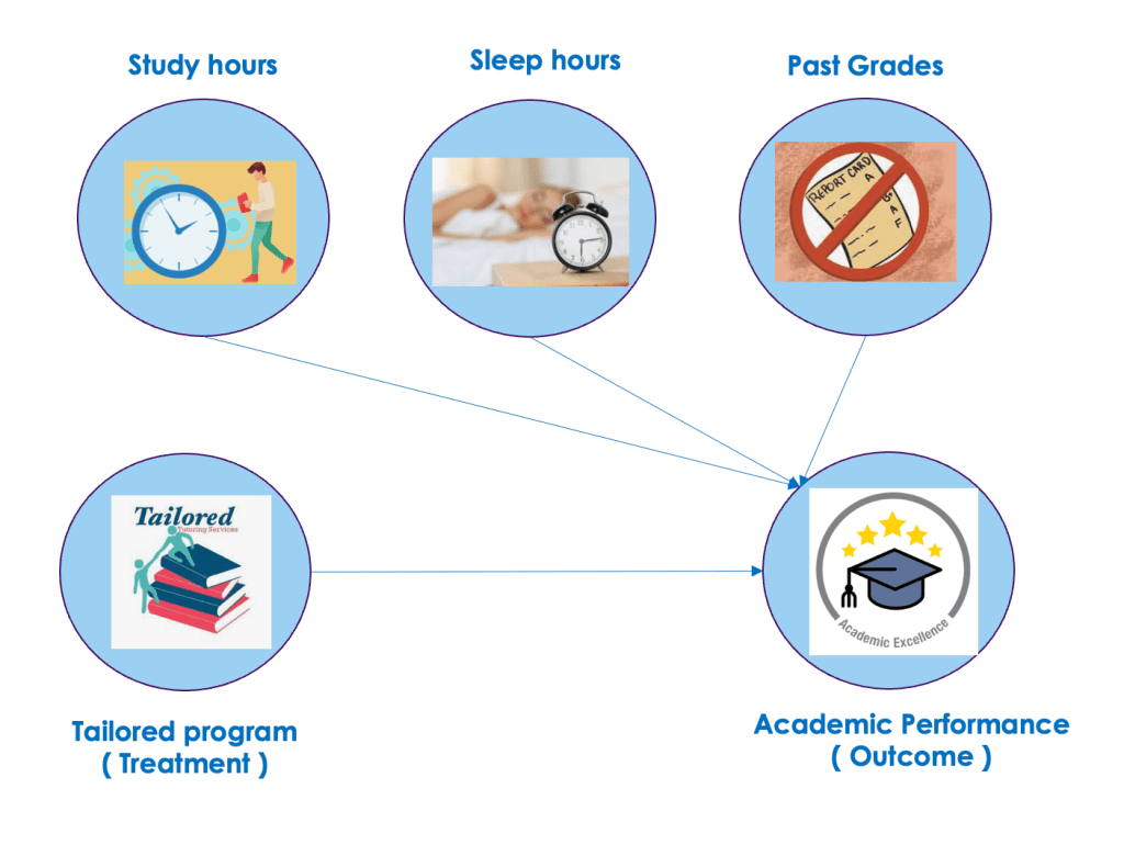
- Effect of instrument on treatment: We analyze how compulsory schooling laws (the instrument variable) affect education (the treatment).
- Estimate the effect of education on outcome: We use the information from the above to estimate how education (treatment) actually affects earnings (outcome), ignoring the influence of natural talent (the unobserved confounders).
By using this method, we can finally isolate the true effect of education on earnings, leaving the confusing influence of natural talent behind. Now, we can confidently answer the question:

Does more education truly lead to a brighter financial future?
Remember, this is just one example, and finding the right instrument variable for your situation can be tricky. But with the right tool in hand, you can navigate the maze of confounding factors and uncover the true causal relationships in your data.
Implementation of Causal estimation using Instrument Variables from scratch

Let us now explain the concept through code. First we will use the linear regression method to take you through the estimation process.
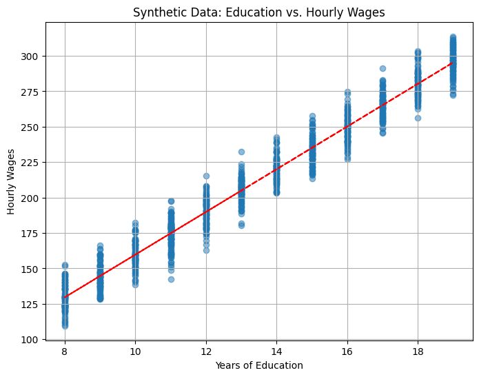
To start off, lets generate some synthetic data set which describes the relationship between the variables.
# Importing the necessary packages
import numpy as np
from sklearn.linear_model import LinearRegression
Now let’s create the synthetic dataset
# Generate sample data (replace with your actual data)
n = 1000
ability = np.random.normal(size=n)
compulsory_schooling = np.random.binomial(1, 0.5, size=n)
education = 5 + 2 * compulsory_schooling + 0.5 * ability + np.random.normal(size=n)
earnings = 10 + 3 * education + 0.8 * ability + np.random.normal(size=n)
This section creates simulated data for n individuals (1000 in this case):
ability: Represents unobserved individual ability (normally distributed).compulsory_schooling: Binary variable indicating whether someone was subject to compulsory schooling (50% chance).education: Years of education, determined by compulsory schooling (2 years difference), ability (0.5 years per unit), and random error.earnings: Annual earnings, influenced by education (3 units per year), ability (0.8 units per unit), and random error.
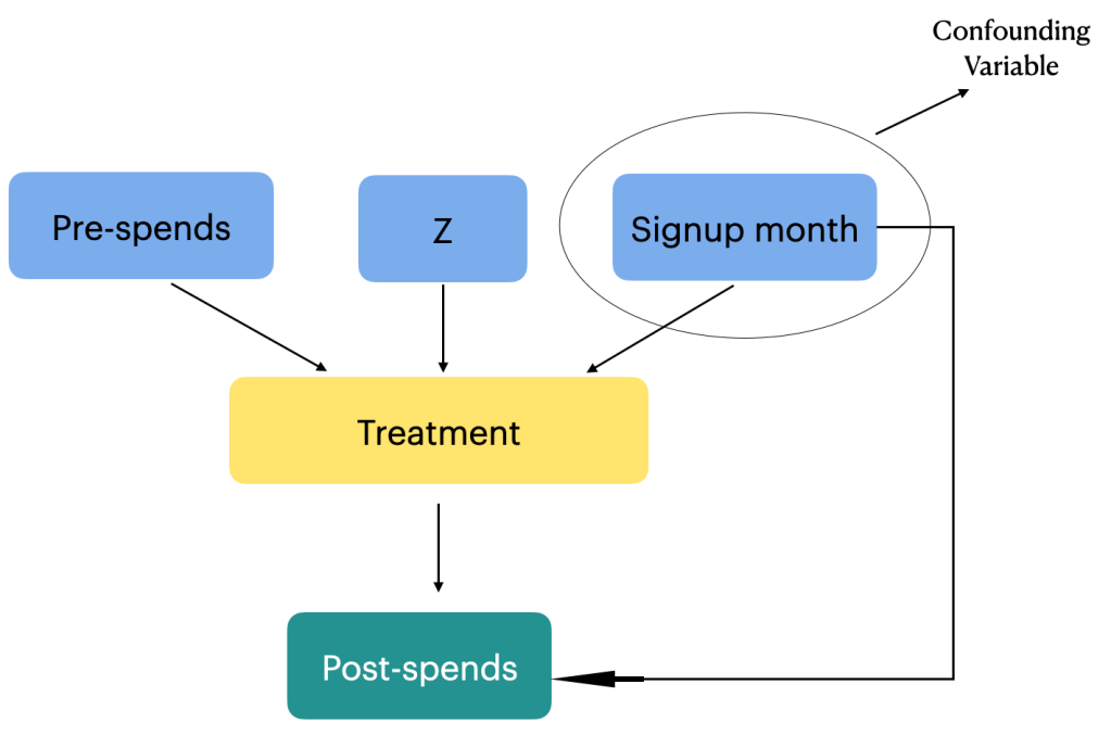
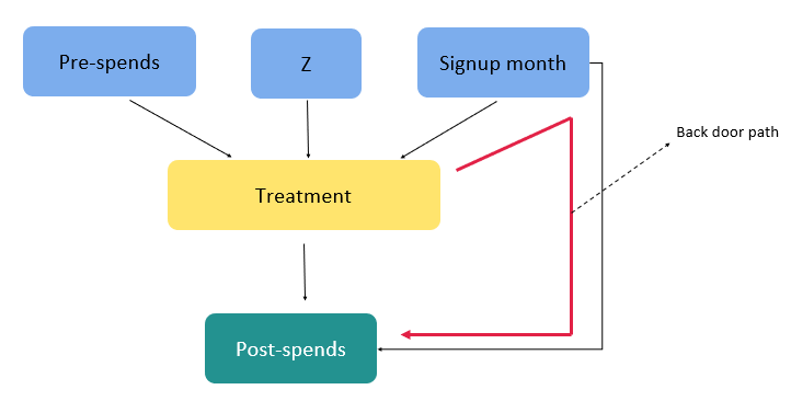
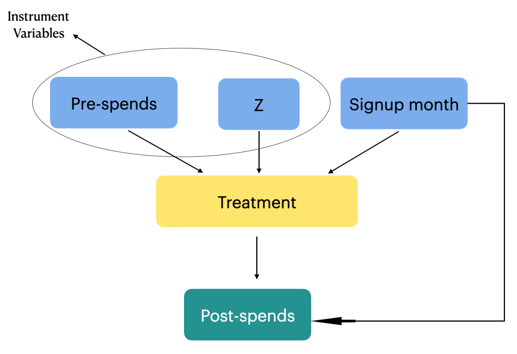
We can see that the variables are defined in such a way that education depends on both schooling laws ( instrument variable) and ability ( unobserved confounder) and the earnings ( outcome ) depends on education ( Treatment ) and ability. The outcome is not directly influenced by the instrument variable, which is one of the condition of selecting an instrument variable.
Let us now implement the first regression model.
# Stage 1: Regress treatment (education) on instrument (compulsory schooling)
stage1_model = LinearRegression()
stage1_model.fit(compulsory_schooling.reshape(-1, 1), education)  # Reshape for 2D input
predicted_education = stage1_model.predict(compulsory_schooling.reshape(-1, 1))
This stage uses linear regression to model how compulsory schooling (compulsory_schooling) affects education (education).
In line 13, we reshape the data to the required 2D format for scikit-learn’s LinearRegression model. The model estimates the effect of compulsory schooling on education, isolating the variation in education directly caused by the instrument (compulsory schooling) and removing the influence of ability (confounding variable).
In line 14, The resulting model predicts the “purified” education values (predicted_education) for each individual, eliminating the confounding influence of ability.
Now that we have found the education variable which is precluded of the influence from unobserved confounder ( ability ), we will build the second regression model.
# Stage 2: Regress outcome (earnings) on predicted treatment from stage 1
stage2_model = LinearRegression()
stage2_model.fit(predicted_education.reshape(-1, 1), earnings)  # Reshape for 2D input
This stage uses linear regression to model how the predicted education (predicted_education) affects earnings (earnings).
Again, in line 16 we reshape the data for compatibility with the model and fit the model to estimate the causal effect of education on earnings. Here we use the “cleaned” education values from stage 1 to isolate the true effect, holding the influence of ability constant.
Let us now extract the coefficients of this model. The coefficient of predicted_education represents the estimated change in earnings associated with a one-unit increase in education, adjusting for the confounding effect of ability.
# Print coefficients (equivalent to summary in statsmodels)
print("Intercept:", stage2_model.intercept_)
print("Coefficient of education:", stage2_model.coef_[0])

Intercept (9.901): This indicates the predicted earnings for someone with zero years of education.
Coefficient of education (3.004): This shows that, on average, each additional year of education is associated with an increase of $3.004 in annual earnings, holding ability constant with the help of the instrument.
Let us try to get some intuition on the exercise we just performed. In the first stage, we estimate how changes in the instrument (here, compulsory schooling laws) impact education. Then in the second stage, we examine how changes in education, predicted from the first stage, impact earnings. The first stage helps address the issue of unobserved confounding by using a variable (the instrument) that only affects the outcome through its impact on the treatment variable. Thus we are able to estimate the real effect of education on the earning capacity, by eliminating any influence from the unobserved confounding variables like ability.
We implemented this exercise using linear regression to get an intuitive understanding of what is going on under the hood. Now let us implement the same exercise using DoWhy library.
5.0 Implementation using DoWhy
We will start by importing the required libraries.
from dowhy import CausalModel
We will be using the same data frame which we used earlier. Let us now define the data frame for our analysis.
# Create a pandas DataFrame
data = pd.DataFrame({
    'ability': ability,
    'compulsory_schooling': compulsory_schooling,
    'education': education,
    'earnings': earnings
})
Next let us define the causal model.
# Define the causal model
model = CausalModel(
    data=data,
    treatment='education',
    outcome='earnings',
    instruments=['compulsory_schooling']
)
The above code creates the causal model using DoWhy.
Let’s break down the key components and the processes happening behind the scenes:
model = CausalModel(...): This line initializes a causal model using the DoWhy library.
data: The dataset containing the variables of interest.
treatment='education': Specifies the treatment variable, i.e., the variable that is believed to have a causal effect on the outcome.
outcome='earnings': Specifies the outcome variable, i.e., the variable whose changes we want to attribute to the treatment.
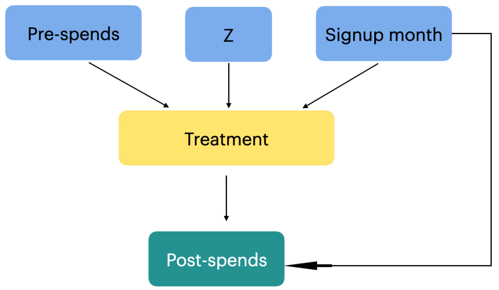
instruments=['compulsory_schooling']: Specifies the instrumental variable(s), if any. In this case, ‘compulsory_schooling’ is used as an instrument.
In the provided code snippet, there is no explicit specification of common causes, which in our case is the variable ‘ability’. The absence of common causes in the CausalModel definition may imply that the common causes are either not considered or are left unspecified. In our case we have said that the common causes or confounders are unobserved. That is why we use the instrument variable ( compulsory_schooling) to negate the effect of unobserved confounders.
When the causal model is defined as shown above, DoWhy performs an identification step where it tries to identify the causal effect using graphical models and do-calculus. It checks if the causal effect is identifiable given the specified variables. To know more about the identification steps you can refer our previous blogs on the subject.
Once identification is successful, the next step is to estimate the causal effect. Let us proceed with the estimation process.
# Identify the causal effect using instrumental variable analysis
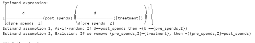
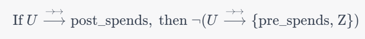
identified_estimand = model.identify_effect(proceed_when_unidentifiable=True)
estimate = model.estimate_effect(identified_estimand, method_name="iv.instrumental_variable")
Line 17 , identified_estimand = model.identify_effect(proceed_when_unidentifiable=True): In this step, the identify_effect method attempts to identify the causal effect based on the specified causal model. The proceed_when_unidentifiable=True parameter allows the analysis to proceed even if the causal effect is unidentifiable, with the understanding that this might result in less precise estimates.
Line 18 estimate = model.estimate_effect(identified_estimand, method_name="iv.instrumental_variable"): This method takes the identified estimand and specifies the method for estimating the causal effect. In this case, the method chosen is instrumental variable analysis, specified by method_name="iv.instrumental_variable". Instrumental variable analysis helps in addressing potential confounding in observational studies by finding an instrument (a variable that is correlated with the treatment but not directly associated with the outcome) to isolate the causal effect.The intuition for the instrument variable was earlier described when we built the linear regression model.
Finally the estimate object contains information about the estimated causal effect. Let us print the causal effect in our case
# Print the causal effect estimate
print("Causal Effect Estimate:", estimate.value)

From the output we can see that its similar to our implementation using the linear regression method. The idea of implementing the linear regression method is to unravel the intuition which is often hidden in black box implementations like that in the DoWhy package.
Now that we have a fair idea and intuition on what is happening in the instrument variable analysis, let us see one more method of implementation called the two-stage least squares (2SLS) regression method. We will be using the statsmodels library for the implementation.
6.0 Ordinary Least Squares (OLS) Method method
Let us see the full implementation using least squares method.
import numpy as np
import pandas as pd
import statsmodels.api as sm

# Set seed for reproducibility
np.random.seed(42)

# Generate synthetic data
n_samples = 1000

# True coefficients
beta_education = 3.5  # True causal effect of education on earnings
gamma_instrument = 2.0  # True effect of the instrument on education
delta_intercept = 5.0  # Intercept in the second stage equation

# Generate data
instrument_z = np.random.randint(0, 2, size=n_samples)  # Instrument (0 or 1)
education_x = 2 * instrument_z + np.random.normal(0, 1, n_samples)  # Education affected by the instrument
earnings_y = delta_intercept + beta_education * education_x + gamma_instrument * instrument_z + np.random.normal(0, 1, n_samples)

# Create a DataFrame
data = pd.DataFrame({'Education': education_x, 'Earnings': earnings_y, 'Instrument': instrument_z})

# First stage regression: Regress education on the instrument
first_stage = sm.OLS(data['Education'], sm.add_constant(data['Instrument'])).fit()
data['Predicted_Education'] = first_stage.predict()

# Second stage regression: Regress earnings on the predicted education
second_stage = sm.OLS(data['Earnings'], sm.add_constant(data['Predicted_Education'])).fit()
In line 6, we set the seed for reproducibility. Then in lines 12-14, we define the true coefficients for the simulation. This step is done only to compare the final results with the actual coefficients, since we have the luxury of defining the data itself.
In lines 17-19, we generate synthetic data for the analysis. The variables for this data are the following.
instrument_zrepresents the instrument (0 or 1).education_xis affected by the instrument.earnings_yis generated based on the true coefficients and some random noise.
In line 22, we create a DataFrame to hold the simulated data.
In lines 25-26, we perform the first stage regression: regress education on the instrument.
sm.OLS: This is creating an Ordinary Least Squares (OLS) regression model. OLS is a method for estimating the parameters in a linear regression model.data['Education']: This is specifying the dependent variable in the regression, which is education (X).sm.add_constant(data['Instrument']): This part is adding a constant term to the independent variable, which is the instrument (Z). The constant term represents the intercept in the linear regression equation..fit(): This fits the model to the data, estimating the coefficients.
We finally store the predictions in a variable ‘Predicted_Eduction‘
In the second stage regression in line 29, earnings is regressed on the predicted education from the first stage.This stage estimates the causal effect of education on earnings, considering the predicted education from the first stage.The coefficient of the predicted education in the second stage represents the causal effect.
Let us look at the results from each stage .
# Print results
print("First Stage Results:")
print(first_stage.summary())

print("\nSecond Stage Results:")
print(second_stage.summary())

Let’s interpret the results obtained from both the first and second stages:
First stage results:
Constant (Intercept): The constant term (const) is estimated to be 0.0462, but its p-value (P>|t|) is 0.308, indicating that it is not statistically significant. This suggests that the instrument is not systematically related to the baseline level of education.
Instrument: The coefficient for the instrument is 1.9882, and its p-value is very close to zero (P>|t| < 0.001). This implies that the instrument is statistically significant in predicting education.
R-squared: The R-squared value of 0.497 indicates that approximately 49.7% of the variability in education is explained by the instrument.
F-statistic:The F-statistic (984.4) is highly significant with a p-value close to zero. This suggests that the instrument as a whole is statistically significant in predicting education.
The overall fit of the first stage regression is reasonably good, given the significant F-statistic and the instrument’s significant coefficient.
The coefficient for the instrument (Z) being 1.9882 with a very low p-value suggests a statistically significant relationship between the instrument (compulsory schooling laws) and education (X). In the context of instrumental variable analysis, this implies that the instrument is a good predictor of the endogenous variable (education) and helps address the issue of endogeneity.
The compulsory schooling laws (instrument) affect education levels. The positive coefficient suggests that when these laws are in place, education levels tend to increase. This aligns with the intuition that compulsory schooling laws, which mandate individuals to stay in school for a certain duration, positively influence educational attainment.
In the context of the broader problem—examining whether education causally increases earnings—the significance of the instrument is crucial. It indicates that the laws that mandate schooling have a significant impact on the educational levels of individuals in the dataset. This, in turn, supports the validity of the instrument for addressing the potential endogeneity of education in the relationship with earnings.
Second stage results:
Constant (Intercept): The constant term (const) is estimated to be 5.0101, and it is statistically significant (P>|t| < 0.001). This represents the baseline earnings when the predicted education is zero.
Predicted Education: The coefficient for predicted education is 4.4884, and it is highly significant (P>|t| < 0.001). This implies that, controlling for the instrument, the predicted education has a positive effect on earnings.
R-squared: The R-squared value of 0.605 indicates that approximately 60.5% of the variability in earnings is explained by the predicted education.
F-statistic: The F-statistic (1530.0) is highly significant, suggesting that the model as a whole is statistically significant in predicting earnings.
The overall fit of the second stage regression is good, with significant coefficients for the constant and predicted education.
The coefficient for predicted education is 4.4884, and its high level of significance (P>|t| < 0.001) indicates that predicted education has a statistically significant and positive effect on earnings. In the second stage of instrumental variable analysis, predicted education is used as the variable to estimate the causal effect of education on earnings while controlling for the instrument (compulsory schooling laws).The intercept (baseline earnings) is also significant, representing earnings when the predicted education is zero.
The positive coefficient suggests that an increase in predicted education is associated with a corresponding increase in earnings. In the context of the overall problem—examining whether education causally increases earnings—this finding aligns with our expectations. The positive relationship indicates that, on average, individuals with higher predicted education levels tend to have higher earnings.
In summary, these results suggest that, controlling for the instrument, there is evidence of a positive causal effect of education on earnings in this example.
7.0 Conclusion
In the course of our exploration of causal estimation in the context of the education and earnings we traversed three distinct methods to unravel the causal dynamics:
Implementation from Scratch using Linear Regression: We embarked on the journey of causal analysis by implementing from scratch using linear regression. This method, was aimed to understand the intuition on the use of instrument variable to estimate the causal link between education and earnings.
Dowhy Implementation: Implementation using DoWhy facilitated a structured causal analysis, allowing us to explicitly define the causal model, identify key parameters, and estimate causal effects. The flexibility and transparency offered by DoWhy proved instrumental in navigating the complexities of causal inference.
Ordinary Least Squares (OLS) Method: We explored the OLS method to enrich our toolkit, for instrumental variable analysis. This method introduced a different perspective, by carefully selecting and leveraging instrumental variables. Employing this method were were able to isolate the causal effect of education on earnings.
Instrumental variable analysis, have impact across diverse domains like finance, marketing, retail,manufacturing etc. Instrumental variable analysis comes into play when we’re concerned about hidden factors affecting our understanding of cause and effect.This method ensures that we get to the real impact of changes or decisions without being misled by other influences. Let us look at its use cases in different domains.

Marketing: In marketing, figuring out the real impact of strategies and campaigns is crucial. Sometimes, it gets complicated because there are hidden factors that can cloud our understanding. Imagine a company launching a new ad approach – instrumental variables, like the reach of the ad, can help cut through the noise, letting marketers see the true effects of the campaign on things like customer engagement, brand perception, and, of course, sales.
Finance: In finance understanding why things happen is a big deal. For example assessing how changes in interest rates affect economic indicators. Instrumental variables help us here, making sure our predictions are solid and helping policymakers and investors make better choices.
Retail: In retail it’s not always clear why people buy what they buy. That’s where instrumental variable analysis can be a handy tool for retailers. Whether it’s figuring out if a new in-store gimmick or a pricing trick really works, instrumental variables, like things that aren’t directly related to what’s happening in the store, can help retailers see what’s really driving customer behavior.
Manufacturing: Making things efficiently in manufacturing involves tweaking a lot of stuff. But how do you know if the latest tech upgrade or a change in how you get materials is actually helping? Enter instrumental variable analysis. It helps you separate the real impact of changes in your manufacturing process from all the other stuff that might be going on. This way, decision-makers can fine-tune their production strategies with confidence.
Instrumental variable analysis helps people in these different fields see things more clearly. It’s not fooled by hidden factors, making it a go-to method for getting to the heart of why things happen in marketing, finance, retail, and manufacturing.
That’s a wrap! But the journey continues…
So, we’ve dipped our toes into the fascinating (and sometimes frustrating) world of causal estimation using instrumental variables. It’s a powerful tool, but it’s not a magic bullet.
The world Causal AI and in general AI is ever evolving, and we’re here to stay ahead of the curve. Want to dive deeper, unlock industry secrets, and gain valuable insights?

Then subscribe to our blog and YouTube channel!
We’ll be serving up fresh content regularly, packed with expert interviews, practical tips, and engaging discussions. Think of it as your one-stop shop for all things business, delivered straight to your inbox and screen. ✨
Click the links below to join the community and start your journey to mastery!
YouTube Channel: [Bayesian Quest YouTube channel]
Remember, the more we learn together, the greater our collective success! Let’s grow, connect, and thrive .
P.S. Don’t forget to share this post with your fellow enthusiasts! Sharing is caring, and we love spreading the knowledge.