

This is the second post of our series on building a self learning recommendation system using reinforcement learning. This series consists of 7 posts where in we progressively build a self learning recommendation system.
- Recommendation system and reinforcement learning primer
- Introduction to multi armed bandit problem ( This post )
- Self learning recommendation system as a bandit problem
- Build the prototype of the self learning recommendation system: Part I
- Build the prototype of the self learning recommendation system: Part II
- Productionising the self learning recommendation system: Part I – Customer Segmentation
- Productionising the self learning recommendation system: Part II – Implementing self learning recommendation
- Evaluating different deployment options for the self learning recommendation systems.
Introduction

In our previous post we introduced different types of recommendation systems and explored some of the basic elements of reinforcement learning. We found out that reinforcement learning problems evaluates different actions when the agent is in a specific state. The action taken generates a certain reward. In other words we get a feedback on how good the action was based on the reward we got. However we wont get the feed back as to whether the action taken was the best available. This is what contrasts reinforcement learning from supervised learning. In supervised learning the feed back is instructive and gives you the quantum of the correctness of an action based on the error. Since reinforcement learning is evaluative, it depends a lot on exploring different actions under different states to find the best one. This tradeoff between exploration and exploitation is the bedrock of reinforcement learning problems like the K armed bandit. Let us dive in.
The Bandit Problem.
In this section we will try to understand K armed bandit problem setting from the perspective of product recommendation.
A recommendation system recommends a set of products to a customer based on the customers buying patterns which we call as the context. The context of the customer can be the segment the customer belongs to, the period in which the customer buys, like which month, which week of the month, which day of the week etc. Once recommendations are made to a customer, the customer based on his or her affinity can take different type of actions i.e. (i) ignore the recommendation (ii) click on the product and further explore (iii) buy the recommended product. The objective of the recommendation system would be to recommend those products which are most likely to be accepted by the customer or in other words maximize the value from the recommendations.
Based on the recommendation example let us try to draw parallels to the K armed bandit. The K-armed bandit is a slot machine which has ‘K’ different arms or levers. Each pull of the lever can have a different outcome. The outcomes can vary from no payoff to winning a jackpot. Your objective is to find the best arm which yields the best payoff through repeated selection of the ‘K’ arms. This is where we can draw parallels’ between armed bandits and recommendation systems. The products recommended to a customer are like the levers of the bandit. The value realization from the recommended products happens based on whether the customer clicks on the recommended product or buys them. So the aim of the recommendation system is to identify the products which will generate the best value i.e which will very likely be bought or clicked by the customer.

Having set the context of the problem statement , we will understand in depth the dynamics of the K-armed bandit problem and couple of solutions for solving them. This will lay the necessary foundation for us to try this in creating our recommendation system.
Non-Stationary Armed bandit problem
When we discussed about reinforcement learning we learned about the reward function. The reward function can be of two types, stationary and non-stationary. In stationary type the reward function will not change over time. So over time if we explore different levers we will be able to figure out which lever gives the best value and stick to it. In contrast,in the non stationary problem, the reward function changes over time. For non stationary problem, identifying the arms which gives the best value will be based on observing the rewards generated in the past for each of the arms. This scenario is more aligned with real life cases where we really do not know what would drive a customer at a certain point of time. However we might be able to draw a behaviour profile by observing different transactions over time. We will be exploring the non-stationary type of problem in this post.
Exploration v/s exploitation

One major dilemma in problems like the bandit is the choice between exploration and exploitation. Let us explain this with our context. Let us say after few pulls of the first four levers we found that lever 3 has been consistently giving good rewards. In this scenario, a prudent strategy would be to keep on pulling the 3rd lever as we are sure that this is the best known lever. This is called exploitation. In this case we are exploiting our knowledge about the lever which gives the best reward. We also call the exploitation of the best know lever as the greedy method.
However the question is, will exploitation of our current knowledge guarantee that we get the best value in the long run ? The answer is no. This is because, so far we have only tried the first 4 levers, we haven’t tried the other levers from 5 to 10. What if there was another lever which is capable of giving higher reward ? How will we identify those unknown high value levers if we keep sticking to our known best lever ? This dilemma is called the exploitation v/s exploration. Having said that, resorting to always exploring will also be not judicious. It is found out that a mix of exploitation and exploration yields the best value over a long run.
Methods which adopt a mix of exploitation and exploration are called ε greedy methods. In such methods we exploit the greedy method most of the time. However at some instances, say with a small probability of ε we randomly sample from other levers also so that we get a mix of exploitation and exploration. We will explore different ε greedy methods in the subsequent sections
Simple averaging method
In our discussions so far we have seen that the dynamics of reinforcement learning involves actions taken from different states yielding rewards based on the state-action pair chosen. The ultimate aim is to maximize the rewards in the long run. In order to maximize the overall rewards, it is required to exploit the actions which gets you the maximum rewards in the long run. However to identify the actions with the highest potential we need to estimate the value of that action over time. Let us first explore one of the methods called simple averaging method.
Let us denote the value of an action (a) at time t as Qt(a). Using simple averaging method Qt(a) can be estimated by summing up all the rewards received for the action (a) divided by the number of times action (a) was selected. This can be represented mathematically as
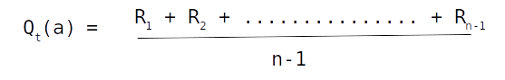
In this equation R1 .. Rn-1 represents the rewards received till time (t) for action (a)
However we know that the estimate of value are a moving average, which means that there would be further instances when action (a) will be selected and corresponding rewards received. However it would be tedious to always sum up all the rewards and then divide it by the number of instances. To avoid such tedious steps, the above equation can be rewritten as follows
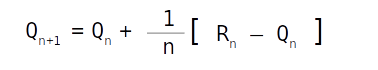
This is a simple update formulae where Qn+1 is the new estimate for the n+1 occurance of action a, Qn is the estimate till the nth try and Rn is the reward received for the nth try .
In simple terms this formulae can be represented as follows
New Estimate <----- Old estimate + Step Size [ Reward - Old Estimate]
For simple averaging method the Step Size is the reciprocal of the number of times that particular action was selected ( 1/n)
Now that we have seen the estimate generation using the simple averaging method, let us look at the complete algorithm.
Initialize values for the bandit arms from 1 to K. Usually we initialize a value of 0 for all the bandit armsDefine matrices to store the Value estimates for all the arms ( Qt(a) ) and initialize it to zeroDefine matrices to store the tracker for all the arms i.e a tracker which stores the number of times each arm was pulledStart a iterative loop andSample a random probability valueif the probability value is greater than ε, pick the arm with the largest value. If the probability value is less than ε, randomly pick an arm.
Get the reward for the selected armUpdate the number tracking matrix with 1 for the arm which was selectedUpdate the Qt(a) matrix, for the arm which was picked using the simple averaging formulae.
Let us look at python implementation of the simple averaging problem next
Implementation of Simple averaging method for K armed bandit
In this implementation we will experiment with around 2000 different bandits with each bandit having 10 arms each. We will be evaluating these bandits for around 10000 steps. Finally we will average the values across all the bandits for each time step. Let us dive into the implementation.
Let us first import all the required packages for the implementation in lines 1-4
import numpy as np
import matplotlib.pyplot as plt
from tqdm import tqdm
from numpy.random import normal as GaussianDistribution
We will start off by defining all the parameters of our bandit implementation. We would have 2000 seperate bandit experiments. Each bandit experiment will run for around 10000 steps. As defined earlier each bandit will have 10 arms. Let us now first define these parameters
# Define the armed bandit variables
nB = 2000 # Number of bandits
nS = 10000 # Number of steps we will take for each bandit
nA = 10 # Number of arms or actions of the bandit
nT = 2 # Number of solutions we would apply
As we discussed in the previous post the way we arrive at the most optimal policy is through the rewards an agent receives in the process of interacting with the environment. The policy defines the actions the agent will take. In our case, the actions we are going to take is the arms which we are going to pull. The reward which we get from our actions is based on the internal calibration of the armed bandit. The policy we will adopt is a mix of exploitation and exploration. This means that most of the time we will exploit the which action which was found to give the best reward. However once in a while we also do a bit of exploration. The exploration is controlled by a parameter ε.
Next let us define the containers to store the rewards which we get from each arm and also to track whether the reward we got was the most optimal reward.
# Defining the rewards container
rewards = np.full((nT, nB, nS), fill_value=0.)
# Defining the optimal selection container
optimal_selections = np.full((nT, nB, nS), fill_value=0.)
print('Rewards tracker shape',rewards.shape)
print('Optimal reward tracker shape',optimal_selections.shape)

We saw earlier that the policy with which we would pull each arm would be a mixture of exploitation and exploration. The way we do exploitation is by looking at the average reward obtained from each arm and then selecting the arm which has the maximum reward. For tracking the rewards obtained from each arm we initialize some values for each of the arm and then store the rewards we receive after each pull of the arm.
To start off we initialize all these values as zero as we don’t have any information about the arms and its reward possibilities.
# Set the initial values of our actions
action_Mental_model = np.full(nA, fill_value=0.0) # action_value_estimates > action_Mental_model
print(action_Mental_model.shape)
action_Mental_model

The rewards generated by each arm of the bandit is through the internal calibration of the bandit. Let us also define how that calibration has to be. For this case we will assume that the internal calibration follows a non stationary process. This means that with each pull of the armed bandit the existing value of the armed bandit is incremented by a small value. The value to increment the internal value of the armed bandits is through a Gaussian process with its mean at 0 and a standard deviation of 1.
As a start we will initialize the calibrated values of the bandit to be zero.
# Initialize the bandit calibration values
arm_caliberated_value = np.full(nA, fill_value=0.0)
arm_caliberated_value

We also need to track how many times a particular action was selected. Therefore we define a counter to store those values.
# Initialize the count of how many times an action was selected
arm_selected_count = np.full(nA, fill_value=0, dtype="int64")
arm_selected_count
The last of the parameters we will define is the exploration probability value. This value defines how often we would be exploring non greedy arms to find their potential.
# Define the epsilon (ε) value
epsilon=0.1
Now we are ready to start our experiments. The first step in the process is to decide whether we want to do exploration or exploitation. To decide this , we randomly sample a value between 0 and 1 and compare it with the exploration probability value ( ε) value we selected. If the sampled value is less than the epsilon value, we will explore, otherwise we will exploit. To explore we randomly choose one of the 10 actions or bandit arms irrespective of the value we know it has. If the random probability value is greater than the epsilon value we go into the exploitation zone. For exploitation we pick the arm which we know generates the maximum reward.
# First determine whether we need to explore or exploit
probability = np.random.rand()
probability
The value which we got is greater than the epsilon value and therefore we will resort to exploitation. If the value were to be less than 0.1 (epsilon value : ε ) we would have explored different arms. Please note that the probability value you will get will be different as this is a random generation process.
Now,let us define a decision mechanism so as to give us the arm which needs to be pulled ( our action) based on the probabiliy value.
# Our decision mechanism
if probability >= epsilon:
  my_action = np.argmax(action_Mental_model)
else:
  my_action = np.random.choice(nA)
print('Selected Action',my_action)
In the above section, in line 31 we check whether the probability we generated is greater than the epsilon value . if It it is greater, we exploit our knowledge about the value of the arms and select the arm which has so far provided the greatest reward ( line 33 ). If the value is less than the epsilon value, we resort to exploration wherein we randomly select an arm as shown in line 35. We can see that the action selected is the first action ( index 0) as we are still in the initial values.
Once we have selected our action (arm) ,we have to determine whether the arm is the best arm in terms of the reward potential in comparison with other arms of the bandit. To do that, we find the arm of the bandit which provides the greatest reward. We do this by taking the argmax of all the values of the bandit as in line 38.
# Find the most optimal arm of the bandits based on its internal calibration calculations
optimal_calibrated_arm = np.argmax(arm_caliberated_value)
optimal_calibrated_arm

Having found the best arm its now time to determine if the value which we as the user have received is equal to the most optimal value of the bandit. The most optimal value of the bandit is the value corresponding to the best arm. We do that in line 40.
# Find the value corresponding to the most optimal calibrated arm
optimal_calibrated_value = arm_caliberated_value[optimal_calibrated_arm]
Now we check if the maximum value of the bandit is equal to the value the user has received. If both are equal then the user has made the most optimal pull, otherwise the pull is not optimal as represented in line 42.
# Check whether the value corresponding to action selected by the user and the internal optimal action value are same.
optimal_pull = float(optimal_calibrated_value == arm_caliberated_value[my_action])
optimal_pull

As we are still on the initial values we know that both values are the same and therefore the pull is optimal as represented by the boolean value 1.0 for optimal pull.
Now that we have made the most optimal pull, we also need to get rewards conssumerate with our action. Let us assume that the rewards are generated from the armed bandit using a gaussian process centered on the value of the arm which the user has pulled.
# Calculate the reward which is a random distribution centered at the selected action value
reward = GaussianDistribution(loc=arm_caliberated_value[my_action], scale=1, size=1)[0]
reward
1.52
In line 45 we generate rewards using a Gaussian distribution with its mean value as the value of the arm the user has pulled. In this example we get a value of around 1.52 which we will further store as the reward we have received. Please note that since this is a random generation process, the values you would get could be different from this value.
Next we will keep track of the arms we pulled in the current experiment.
# Update the arm selected count by 1
arm_selected_count[my_action] += 1
arm_selected_count

Since the optimal arm was the first arm, we update the count of the first arm as 1 as shown in the output.
Next we are going to update our estimated value of each of the arms we select. The values we will be updating will be a function of the reward we get and also the current value it already has. So if the current value is Vcur, then the new value to be updated will be Vcur + (1/n) * (r - Vcur) where n is the number of times we have visited that particular arm and 'r' the reward we have got for pulling that arm.
To calcualte this updated value we need to first find the following values
Vcur and n . Let us get those values first
Vcur would be estimated value corresponding to the arm we have just pulled
# Get the current value of our action
Vcur = action_Mental_model[my_action]
Vcur
0.0
n would be the number of times the current arm was pulled
# Get the count of the number of times the arm was exploited
n = arm_selected_count[my_action]
n
1
Now we will update the new value against the estimates of the arms we are tracking.
# Update the new value for the selected action
action_Mental_model[my_action] = Vcur + (1/n) * (reward - Vcur)
action_Mental_model

As seen from the output the current value of the arm we pulled is updated in the tracker. With each successive pull of the arm, we will keep updating the reward estimates. After updating the value generated from each pull the next task we have to do is to update the internal calibration of the armed bandit as we are dealing with a non stationary value function.
# Increment the calibration value based on a Gaussian distribution
increment = GaussianDistribution(loc=0, scale=0.01, size=nA)
# Update the arm values with the updated value
arm_caliberated_value += increment
# Updated arm value
arm_caliberated_value

As seen from lines 59-64, we first generate a small incremental value from a Gaussian distribution with mean 0 and standard deviation 0.01. We add this value to the current value of the internal calibration of the arm to get the new value. Please note that you will get a different value for these processes as this is a random generation of values.
These are the set of processes for one iteration of a bandit. We will continue these iterations for 2000 bandits and for each bandit we will iterate for 10000 steps. In order to run these processes for all the iterations, it is better to represent many of the processes as separate functions and then iterate it through. Let us get going with that task.
Function 1 : Function to select actions
The first of the functions is the one to generate the actions we are going to take.
def Myaction(epsilon,action_Mental_model):
    probability = np.random.rand()
    if probability >= epsilon:
        return np.argmax(action_Mental_model)

    return np.random.choice(nA)
Function 2 : Function to check whether action is optimal and generate rewards
The next function is to check whether our action is the most optimal one and generate the reward for our action.
def Optimalaction_reward(my_action,arm_caliberated_value):
  # Find the most optimal arm of the bandits based on its internal calibration calculations
  optimal_calibrated_arm = np.argmax(arm_caliberated_value)
  # Then find the value corresponding to the most optimal calibrated arm
  optimal_calibrated_value = arm_caliberated_value[optimal_calibrated_arm]
  # Check whether the value of the test bed corresponding to action selected by the user and the internal optimal action value of the test bed are same.
  optimal_pull = float(optimal_calibrated_value == arm_caliberated_value[my_action])
  # Calculate the reward which is a random distribution centred at the selected action value
  reward = GaussianDistribution(loc=arm_caliberated_value[my_action], scale=1, size=1)[0]
  return optimal_pull,reward
Function 3 : Function to update the estimated value of arms of the bandit
def updateMental_model(my_action, reward,arm_selected_count,action_Mental_model):
  # Update the arm selected count with the latest count
  arm_selected_count[my_action] += 1
  # find the current value of the arm selected
  Vcur = action_Mental_model[my_action]
  # Find the number of times the arm was pulled
  n = arm_selected_count[my_action]
  # Update the value of the current arm
  action_Mental_model[my_action] = Vcur + (1/n) * (reward - Vcur)
  # Return the arm selected and our mental model
  return arm_selected_count,action_Mental_model
Function 4 : Function to increment reward values of the bandits
The last of the functions is the function we use to make the reward generation non-stationary.
def calibrateArm(arm_caliberated_value):
    increment = GaussianDistribution(loc=0, scale=0.01, size=nA)
    arm_caliberated_value += increment
    return arm_caliberated_value
Now that we have defined the functions, we will use these functions to iterate through different bandits and multiple steps for each bandit.
for nB_i in tqdm(range(nB)):
  # Initialize the calibration values for the bandits
  arm_caliberated_value = np.full(nA, fill_value=0.0)
  # Set the initial values of the mental model for each bandit
  action_Mental_model = np.full(nA, fill_value=0.0)
  # Initialize the count of how many times an arm was selected
  arm_selected_count = np.full(nA, fill_value=0, dtype="int64")
  # Define the epsilon value for probability of exploration
  epsilon=0.1
  for nS_i in range(nS):
    # First select an action using the helper function
    my_action = Myaction(epsilon,action_Mental_model)
    # Check whether the action is optimal and calculate the reward
    optimal_pull,reward = Optimalaction_reward(my_action,arm_caliberated_value)
    # Update the mental model estimates with the latest action selected and also the reward received
    arm_selected_count,action_Mental_model = updateMental_model(my_action, reward,arm_selected_count,action_Mental_model)
    # store the rewards
    rewards[0][nB_i][nS_i] = reward
    # Update the optimal step selection counter
    optimal_selections[0][nB_i][nS_i] = optimal_pull
    # Recalibrate the bandit values
    arm_caliberated_value = calibrateArm(arm_caliberated_value)
In line 96, we start the first iterative loop to iterate through each of the set of bandits . Lines 98-104, we initialize the value trackers of the bandit and also the rewards we receive from the bandits. Finally we also define the epsilon value. From lines 105-117, we carry out many of the processes we mentioned earlier like
- Selecting our action i.e the arm we would be pulling ( line 107)
- Validating whether our action is optimal or not and getting the rewards for our action ( line 109)
- Updating the count of our actions and updating the rewards for the actions ( line 111 )
- Store the rewards and optimal action counts ( lines 113-115)
- Incrementing the internal value of the bandit ( line 117)
Let us now run the processes and capture the values.

Let us now average the rewards which we have got accross the number of bandit experiments and visualise the reward trends as the number of steps increase.
# Averaging the rewards for all the bandits along the number of steps taken
avgRewards = np.average(rewards[0], axis=0)
avgRewards.shape

plt.plot(avgRewards, label='Sample weighted average')
plt.legend()
plt.xlabel("Steps")
plt.ylabel("Average reward")
plt.show()

From the plot we can see that the average value of rewards increases as the number of steps increases. This means that with increasing number of steps, we move towards optimality which is reflected in the rewards we get.
Let us now look at the estimated values of each arm and also look at how many times each of the arms were pulled.
# Average rewards received by each arm
action_Mental_model

From the average values we can see that the last arm has the highest value of 1.1065. Let us now look at the counts where these arms were pulled.
# No of times each arm was pulled
arm_selected_count

From the arm selection counts, we can see that the last arm was pulled the maximum. This indicates that as the number of steps increased our actions were aligned to the arms which gave the maximum value.
However even though the average value increased with more steps, does it mean that most of the times our actions were the most optimal ? Let us now look at how many times we selected the most optimal actions by visualizing the optimal pull counts.
# Plot of the most optimal actions
average_run_optimality = np.average(optimal_selections[0], axis=0)
average_run_optimality.shape
plt.plot(average_run_optimality, label='Simple weighted averaging')
plt.legend()
plt.xlabel("Steps")
plt.ylabel("% Optimal action")
plt.show()

From the above plot we can see that there is an increase in the counts of optimal actions selected in the initial steps after which the counts of the optimal actions, plateau’s. And finally we can see that the optimal actions were selected only around 40% of the time. This means that even though there is an increasing trend in the reward value with number of steps, there is still room for more value to be obtained. So if we increase the proportion of the most optimal actions, there would be a commensurate increase in the average value which will be rewarded by the bandits. To achieve that we might have to tweak the way how the rewards are calculated and stored for each arm. One effective way is to use the weighted averaging method
Weighted Averaging Method
When we were dealing with the simple averaging method, we found that the update formule was as follows
New Estimate <----- Old estimate + Step Size [ Reward - Old Estimate]
In the formule, the Step Size for simple averaging method is the reciprocal of the number of times that particular action was selected ( 1/n)
In weighted averaging method we make a small variation in the step size. In this method we use a constant step size method called alpha. The new update formule would be as follows
Qn+1 = Qn + alpha * (reward - Qn)
Usually we take some small values of alpha less than 1 say 0.1 or 0.01 or values similar to that.
Let us now try the weighted averaging method with a step size of 0.1 and observe what difference this method have on the optimal values of each arm.
In the weighted averaging method all the steps are the same as the simple averaging, except for the arm update method which is a little different. Let us define the new update function.
def updateMental_model_WA(my_action, reward,action_Mental_model):
  alpha=0.1
  qn = action_Mental_model[my_action]
  action_Mental_model[my_action] = qn + alpha * (reward - qn)
  return action_Mental_model
Let us now run the process again with the updated method. Please note that we store the values in the same rewards and optimal_selection matrices. We store the value of weighted average method in index [1]
for nB_i in tqdm(range(nB)):
  # Initialize the calibration values for the bandits
  arm_caliberated_value = np.full(nA, fill_value=0.0)
  # Set the initial values of the mental model for each bandit
  action_Mental_model = np.full(nA, fill_value=0.0)
  # Define the epsilon value for probability of exploration
  epsilon=0.1
  for nS_i in range(nS):
    # First select an action using the helper function
    my_action = Myaction(epsilon,action_Mental_model)
    # Check whether the action is optimal and calculate the reward
    optimal_pull,reward = Optimalaction_reward(my_action,arm_caliberated_value)
    # Update the mental model estimates with the latest action selected and also the reward received
    action_Mental_model = updateMental_model_WA(my_action, reward,action_Mental_model)
    # store the rewards
    rewards[1][nB_i][nS_i] = reward
    # Update the optimal step selection counter
    optimal_selections[1][nB_i][nS_i] = optimal_pull
    # Recalibrate the bandit values
    arm_caliberated_value = calibrateArm(arm_caliberated_value)

Let us look at the plots for the weighted averaging method.
average_run_rewards = np.average(rewards[1], axis=0)
average_run_rewards.shape
plt.plot(average_run_rewards, label='weighted average')

plt.legend()
plt.xlabel("Steps")
plt.ylabel("Average reward")
plt.show()

From the plot we can see that the average reward increasing with number of steps. We can also notice that the average values obtained higher than the simple averaging method. In the simple averaging method the average value was between 1 and 1.2. However in the weighted averaging method the average value reaches within the range of 1.2 to 1.4. Let us now see how the optimal pull counts fare.
average_run_optimality = np.average(optimal_selections[1], axis=0)
average_run_optimality.shape
plt.plot(average_run_optimality, label='Weighted averaging')
plt.legend()
plt.xlabel("Steps")
plt.ylabel("% Optimal action")
plt.show()

We can observe from the above plot that we take the optimal action for almost 80% of the time as the number of steps progress towards 10000. If you remember the optimal action percentage was around 40% for the simple averaging method. The plots show that the weighted averaging method performs better than the simple averaging method.
Wrapping up
In this post we have understood two methods of finding optimal values for a K armed bandit. The solution space is not limited to these two methods and there are many more methods for solving the bandit problem. The list below are just few of them
- Upper Confidence Bound Algorithm ( UCB )
- Bayesian UCB Algorithm
- Exponential weighted Algorithm
- Softmax Algorithm
Bandit problems are very useful for many use cases like recommendation engines, website optimization, click through rate etc. We will see more use cases of bandit algorithm in some future posts
What next ?
Having understood the bandit problem, our next endeavor would be to use the concepts in building a self learning recommendation system. The next post would be a pre-cursor to that. In the next post we will formulate our problem context and define the processes for building the self learning recommendation system using a bandit algorithm. This post will be released next week ( Jan 17th 2022).
Please subscribe to this blog post to get notifications when the next post is published.
You can also subscribe to our Youtube channel for all the videos related to this series.
The complete code base for the series is in the Bayesian Quest Git hub repository
Do you want to Climb the Machine Learning Knowledge Pyramid ?
Knowledge acquisition is such a liberating experience. The more you invest in your knowledge enhacement, the more empowered you become. The best way to acquire knowledge is by practical application or learn by doing. If you are inspired by the prospect of being empowerd by practical knowledge in Machine learning, subscribe to our Youtube channel
I would also recommend two books I have co-authored. The first one is specialised in deep learning with practical hands on exercises and interactive video and audio aids for learning
This book is accessible using the following links
The Deep Learning Workshop on Amazon
The Deep Learning Workshop on Packt
The second book equips you with practical machine learning skill sets. The pedagogy is through practical interactive exercises and activities.

This book can be accessed using the following links
The Data Science Workshop on Amazon
The Data Science Workshop on Packt
Enjoy your learning experience and be empowered !!!!
.
