Build you Computer Vision Application – Part VI: Road pothole detector using Tensorflow Object Detection API

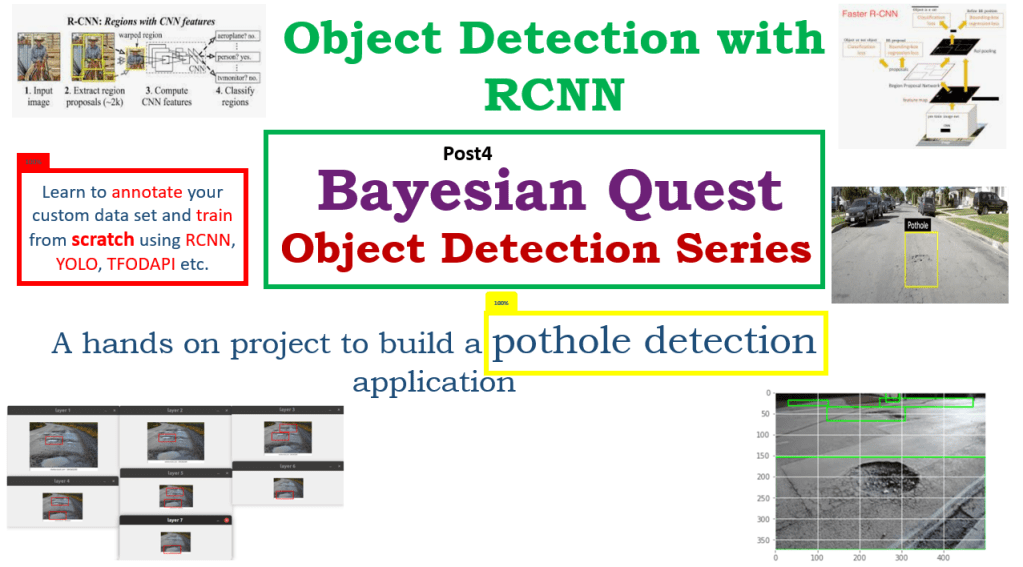
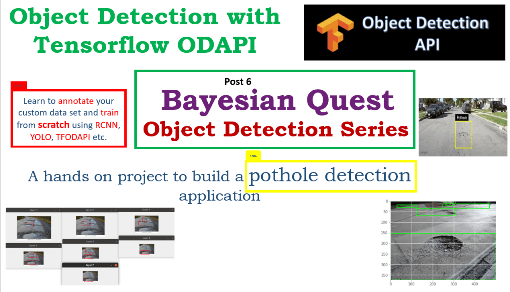
This is the sixth post of the series were we build a road sign and pothole detection application. We will be using multiple methods through out this series which includes computer vision techniques using opencv, annotating images using labelImg, mastering Tensorflow object detection API, Training objection detection using transfer learning, Object detection on video etc. This series will be split across 8 posts.

1. Introduction to object detection

2. Data set preparation and annotation Using LabelImg

3. Building your object detection model from scratch using Image pyramids and sliding window

4. Building your road pothole detector using RCNN

5. Building your road pothole detector using YOLO

6. Building you road pothole detector using Tensorflow object detection API ( This Post)

7. Building your video analytics application for detecting potholes

8. Deploying your video analytics application for detection of potholes

In this post we will discuss in detail the process for training an object detector using the Tensorflow Object Detection API(TFODAPI).

Introduction

Over the past few posts of this series we explored many frameworks through which we created object detection models to detect potholes on road. All the frameworks which we explored till post 5 were about some specific type of model. However in this post we are going to do something different. In this post we will learn about a great utility to do object detection and its called Tensorflow Object Detection API ( TFODAPI ). This is a great API with which we would be able to train custom object detection models using different types of networks. In this post we will use TFODAPI to build our pothole detector. Let us dive in.

Installation of Tensorflow Object Detection API

The pre-requisite for Tensorflow Object Detection is the installation of Tensorflow. To install Tensorflow on your machine you can follow the following link.

Once Tensorflow is installed, we can proceed with the installation of TFODAPI . This installation has 4 major steps.

  1. Downloading Tensorflow model garden
  2. Protobut installation / compilation
  3. COCO API installation
  4. Install object detection API.

You can do these step wise installation using the following link.

If the installation steps are correct, on testing your installation you should get the following screen

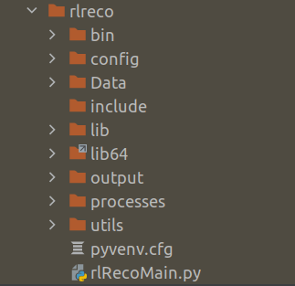
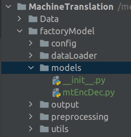
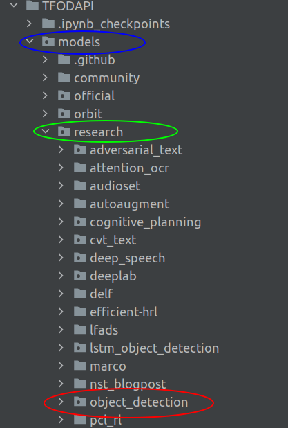
Once all the installations are correct you will have the following folder structure.

Please note that in the installation link provided above, the root folder would be named as 'Tensorflow', however in the installation followed here the root folder is named as 'TFODAPI'. Other than that, the important folder which you need to verify is the /models folder and the other folders created under it. Once this structure is in place, we can get into the next step which is to start the training process using the Custom object detector.

Training a Custom Object detector

Having installed the Tensorflow object detection API, its now the time to get to the training process. In the training process we will be covering the following processes

  • Create the workspace for training
  • Generate tf records from the annotated dataset
  • Configure the training pipeline and monitor progress
  • Export the resulting model and use it to detect porholes

Let us start with the first process

Workspace for training

We start off, creating the following sub-folders within our existing folder structure.

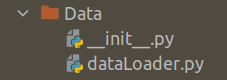
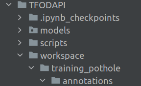
We first create a folder called workspace, under the TFODAPI folder. The workspace folder is where we keep all the training configurations. Let us look at the subfolders of the workspace folder.

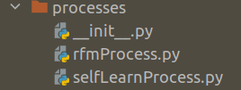
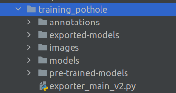
training_pothole : This folder is where the training process gets implemented. Each time we do a training, it is advisable to create a new training_pothole subfolder. This folder has different subfolders under it as follows.

annotations : This folder will contain the train and test data in a format called tf.records. We will see how to create the tf.records in short while.

exported-models :After the training is complete we export the model object to do inference using the train model. This folder will contain the model we will use for inference.

images : This folder contains the raw train and test images which we want to train.

models : This folder will contain a subfolder for each training job we implement. For example, I have created the current training using a ssd_resnet50 model. So you will find a folder related to that as shown in the image below

Once the training is initiated you will have all the training related checkpoints and also the *.config file which contains all the parameters within this subfolder.

pre-trained-models : This folder contains the pre-trained models which we use to initiate our training process. So every type of pretrained model we use will be in a separate subfolder as shown in the image below.

These are the different folders which you will have to create to initiate the training process.

Having seen all the constituent folders within the workspace, let us now get into the training process. As a first step in the training process, let us create the train and test records.

Creating train and test records

Before creating the train and test records, we will have to split the total data into train and test sets using the train_test_split function in scikit learn. After creating the train and test sets, we will move those files inside the train and test folders which are within the images folder. We will do all these processes in the Jupyter notebook.

We will start by importing the necessary library files

import glob
import pandas as pd
import os
import random
from sklearn.model_selection import train_test_split
import shutil

Next let us change our current directory in the Jupyter notebook to the TFODAPI directory. Please note that you will have to give the correct path where your root folder lies instead of the path which is represented here below

!cd /BayesianQuest/Pothole/TFODAPI

Let us also list down all the images we annotated in post 2. We will be using the same set of images in this post.

# List down all the annotated images
random.seed(123)
# Initialize the folder where the annotated images are placed
datafolder = '/BayesianQuest/Pothole/data/annotatedImages'
# List down all the images in the data folder
images = glob.glob(datafolder + '/*.jpeg')
print(len(images))
images

As seen in the output, I have taken around 18 images for this process. The number of images you want to use, is your prerogative, more the better.

Let us now sort the images and the split the data into train and test sets.

# Let us sort the images and the split it into train and test sets
images.sort()

# Split the dataset into train-valid-test splits 
train_images, test_images = train_test_split(images,test_size = 0.1, random_state = 123)

print('Total train images :',len(train_images))
print('Total test images:',len(test_images))

After having split the data into train and test sets, we need to move the files into the images folder . We need to create two folders under the images folder and name them train and test.

# Creating the train and test folders inside the workspace images folder
!mkdir workspace/training_pothole/images/train workspace/training_pothole/images/test

Now that we have the train and test folders created let us move the files to the destination folders . We will move the file using the below function.

#Utility function to move images 
def move_files_to_folder(list_of_files, destination_folder):
    for f in list_of_files:
        try:
            shutil.move(f, destination_folder)
        except:
            print(f)
            assert False

Let us move the files using the above function

# Move the splits into their folders
move_files_to_folder(train_images, 'workspace/training_pothole/images/train')
move_files_to_folder(test_images, 'workspace/training_pothole/images/test/')

Next we will explore the creation of tf records, a format which is required to read data into TFODAPI.

Creation of tf.records file from the images

In this section we will switch gears and then go about executing the next process in python scripts.

When initiating training, we will be using many pre-defined methods and classes which comes with the API. Most of them are within the models/research/object_detection folder in our root folder,TFODAPI, as shown below

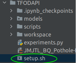
To utilise them in our training and inference scripts, we need to add those paths in the environment. In linux this can be easily be enabled by running those paths in a shell script ( .sh files). Let us first create a shell script to access all these paths.

Open a text editor,create a file called setup.sh and add the following lines in the file

#!/bin/sh
export  PYTHONPATH=$PYTHONPATH:/BayesianQuest/Pothole/TFODAPI/models/research:/BayesianQuest/Pothole/TFODAPI/models/research/slim

This file basically contains the path to the TFODAPI/models/research and TFODAPI/models/research/slim path. The path to the TFODAPI must be changed according to your specific paths. Also please note that you need to have the script export and the paths in the same line.

For Windows system, you can add these paths to the environment variables.

Once the file is created, save that in the folder TFODAPI as shown below

To execute the shell script, open a terminal and the execute the following commands

There will not be any message or output after executing this script. You will be returned to your terminal prompt after execution.

This will ensure that all the paths are entered as environment variables.

Creation of label maps

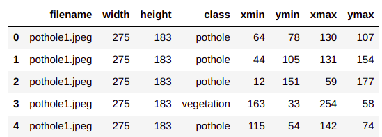
TFODAPI requires a label map, which maps each of the labels to an integer value. This label map is used both by the training and detection processes. The mapping is based on the number of classes we have in the pothole_df.csv file we created in post2 of this series.

# Reading the csv file
pothole_df = pd.read_csv('../pothole_df.csv')
pothole_df.head()
pothole_df['class'].unique()

To create a label map open a text editor, name it label_map.pbtxt and include the below mapping in that file.

item {
    id: 1
    name: 'pothole'
}
item {
    id: 2
    name: 'vegetation'
}
item {
    id: 3
    name: 'sign'
}
item {
    id: 4
    name: 'vehicle'
}

This has to be placed in the folder ‘annotation’ in our workspace.

Creation of tf.records

Now we have all the required files to create our tf.records. Let us open the text editor, name it generate_tfrecord.py and insert the following code.

import os
import glob
import pandas as pd
import io
os.environ['TF_CPP_MIN_LOG_LEVEL'] = '2'    # Suppress TensorFlow logging (1)
import tensorflow.compat.v1 as tf
import argparse
from PIL import Image
from object_detection.utils import dataset_util, label_map_util


# Define the argument parser
arg = argparse.ArgumentParser()
arg.add_argument("-l","--labels-path",help="Path to the labels .pbxtext file",type=str)
arg.add_argument("-o","--output-path",help="Path to the output .tfrecord file",type=str)
arg.add_argument("-i","--image_dir",help="Path to the folder where the input image files are stored. ", type=str, default=None)
arg.add_argument("-a","--anot_file",help="Path to the folder where the annotation file is stored. ", type=str, default=None)

args = arg.parse_args()

# Load the labels files
label_map = label_map_util.load_labelmap(args.labels_path)
label_map_dict = label_map_util.get_label_map_dict(label_map)

# Function to extract information from the images
def create_tf_example(path,annotRecords):
    with tf.gfile.GFile(path, 'rb') as fid:
        encoded_jpg = fid.read()
    encoded_jpg_io = io.BytesIO(encoded_jpg)
    image = Image.open(encoded_jpg_io)
    width, height = image.size
    # Get the filename from the path
    filename = path.split("/")[-1].encode('utf8')
    image_format = b'jpeg'
    # Get all the lists to store the records
    xmins = []
    xmaxs = []
    ymins = []
    ymaxs = []
    classes_text = []
    classes = []
    # Iterate through the annotation records and collect all the records
    for index, row in annotRecords.iterrows():
        xmins.append(row['xmin'] / width)
        xmaxs.append(row['xmax'] / width)
        ymins.append(row['ymin'] / height)
        ymaxs.append(row['ymax'] / height)
        classes_text.append(row['class'].encode('utf8'))
        classes.append(label_map_dict[row['class']])
    # Store all the examples in the format we want
    tf_example = tf.train.Example(features=tf.train.Features(feature={
        'image/height': dataset_util.int64_feature(height),
        'image/width': dataset_util.int64_feature(width),
        'image/filename': dataset_util.bytes_feature(filename),
        'image/source_id': dataset_util.bytes_feature(filename),
        'image/encoded': dataset_util.bytes_feature(encoded_jpg),
        'image/format': dataset_util.bytes_feature(image_format),
        'image/object/bbox/xmin': dataset_util.float_list_feature(xmins),
        'image/object/bbox/xmax': dataset_util.float_list_feature(xmaxs),
        'image/object/bbox/ymin': dataset_util.float_list_feature(ymins),
        'image/object/bbox/ymax': dataset_util.float_list_feature(ymaxs),
        'image/object/class/text': dataset_util.bytes_list_feature(classes_text),
        'image/object/class/label': dataset_util.int64_list_feature(classes),
    }))

    return tf_example


def main(_):

    # Create the writer object
    writer = tf.python_io.TFRecordWriter(args.output_path)
    # Get the annotation file from the arguments
    annotFile = pd.read_csv(args.anot_file)
    # Get the path to the image directory
    path = os.path.join(args.image_dir)
    # Get the list of all files in the image directory
    imgFiles = glob.glob(path + "/*.jpeg")
    # Read each of the file and then extract the details
    for imgFile in imgFiles:
        # Get the file name from the path
        fname = imgFile.split("/")[-1]        
        # Get all the records for the filename from the annotation file
        annotRecords = annotFile.loc[annotFile.filename==fname,:]
        tf_example =  create_tf_example(imgFile,annotRecords)
        # Write the records to the required format
        writer.write(tf_example.SerializeToString())
    writer.close()
    print('Successfully created the TFRecord file: {}'.format(args.output_path))
if __name__ == '__main__':
    tf.app.run()

Lines 1-9, we import the necessary library files and in lines 13-19 we define the arguments.

In line 14, we define the path to the label map file ( .pbtxt ) file we created earlier

We define the path where we will be writing the .tfrecord file in line 15. In our case this is the path to the annotations folder.

The next argument we provide in line 16, is the path to the images folder. Here we give either the train folder or test folder.

The final argument, in line 17 is the path to the annotation file i.e pothole_df.csv file.

Next task is to process the label mapping file we created. For processing this file we use two utility functions which are part of the Tensorflow Object detection API, which we imported in line 9. After the processing in line 23, we get a label map dictionary, which is further used in creation of the tf.records files.

In lines 26-67, is a function used for extracting features from the images and the label maps to create the tf.record. Let us look at the function

The parameters to the function are the following

path : This is the path to the image we are going to process

annotRecords : This is the row of the pothole_df.csv file which contains information of the image and the bounding boxes in that image.

Moving on inside the function lines 26-29 implements a module tf.io.gfile for reading the input image file. This module provides an API that is close to Python’s file I/O object. TensorFlow exports these objects as tf.io.gfile, so that you can use these implementations for saving and loading checkpoints, writing to TensorBoard logs, and accessing training data.

In lines 30-31, the image is opened and its dimensions are read.

The filename is extracted from the path in line 33 and in line 34 the file format is defined.

Lines 36-49, extracts the bounding box information in the respective lists and also stores the class name in the string format and also the numerical format from the label map.

Finally in lines 51-63, all these information extracted from the images and its class names are stored in a format called tf.train.Example. Once these information are packed in the tf.train.Example object it gets written to the tf. record format. That takes us to the end of the function and now we will see the complete process , where this function will be called to extract information from the images.

Lines 72-89, is where the process gets executed. Let us see them line by line.

In line 72, the writer is defined using the TfRecordWriter() method and is written to the output folder to the .record format ( for eg. train.record / test.record)

We read the annotation csv file in line 74 and then extracts the path to the image directory in line 76 and lists down all the the image paths in line 78.

We then iterate through each of the image path in line 80 for further feature extraction within the iterative loop.

We extract the file name from the path in line 82 and the get all the annotation information for the file from the annotation csv file in line 84

We extract all the information of the file in line 85 using the create_tf_example() function we saw earlier and get the tf_example object. This object is finally written as a string in the .record in line 87

The writer object is closed after all the image files are processed.

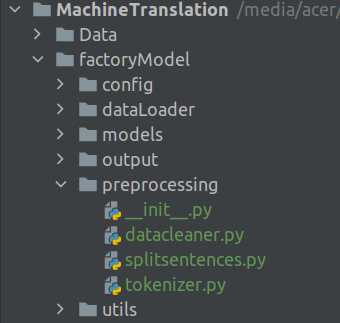
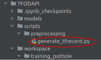
We will save the generate_tfrecord.py in the scripts/preprocessing folder as shown below

To run the file, we will open a terminal and then execute the command in the following format.

$ python generate_tfrecord.py -i [path to images folder] -a [path to annotation csv file] -l [path to label map .pbtxt file] -o [path to the output folder where .record files are written]

For example

Need to run this command for both the train images and test images seperately. Need to change the path of the files folder and also .record name based on whether it is train or test. Once these scripts are executed you will find the train.record and test.record files in the annotation folder as shown below.

That takes us to the end of train and test record processing steps. Next we will start the training process.

Training the Pothole Detection model using pre-trained model

We will not be training the model from scratch, rather we would be fine tuning a pre-trained model for our purpose. The pre-trained model we will be using would be SSD ResNet50 V1 FPN 640×640. These pre-trained models are available in TensorFlow 2 Detection Model Zoo. Later on I would encourage you to implement the same detector using a Faster RCNN model from this repository.

We start our training process by downloading the model we want to implement from the TensorFlow 2 Detection Model Zoo.

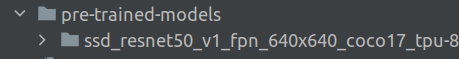
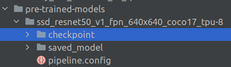
Once we click on the link, a .tar.gz file gets downloaded to your local drive. Extract the contents of the tar file and then move the complete folder into the folder pre-trained-models. Since we extracted the model SSD ResNet50 V1 FPN 640×640, our folder, pre-trained-models will have the following structure.

The more models you want to download, you need to maintain seperte folder structure for each of the model you want to use. I have downloded the Faster RCNN model also, and now the structure looks like the following.

Creating the training pipeline

After unloading the contents of the model to the pre-trained models folder, we will now create a new folder under the folder workspace/training_pothole/models and name it my_ssd_resnet50_v1_fpn and then copy the pipeline.config file from the folder pre-trained-models/ssd_resnet50_v1_fpn_640x640_coco17_tpu-8 and place it in the new folder my_ssd_resnet50_v1_fpn you created. Now the structure will look like the below.

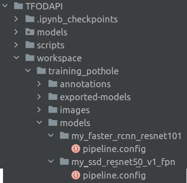
Please note that I also have faster_rcnn model here. So for each model you download the structure will look like the above.

Now that we have copied the pipeline.config file, we will have to make changes to the file to cater to our specific purpose.

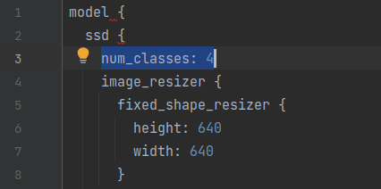
  • Change 1 : The first change we have to make is in line 3 for the number of classes. We need to change the number of classes to 4
  • Change 2 : The next change is in line 131 for the batch size. Depending on the number of examples, you need to change the batch size.
  • Change 3 : The next optional change is for the number of training steps as in line 152 and 154. Depending on the configuration of your machine you can change it to the number of steps you want to train the model.
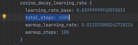
  • Change 4 : Path to the check point of the pre-trained model in line 161
  • Change 5 : Change the fine tune checkpoint type to “detection” from the default “classification'” in line 167
  • Change 6 : label_map_path and train record paths , line 172 and 174
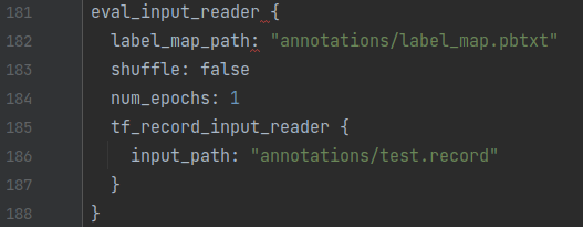
  • Change 7: label_map_path and test record paths, line 182 and 186

Now that the config file is customised, its time to start our training process.

Training the model

We have a script which is part of the API to do the training. This can be copied from the folder TFODAPI/models/research/object_detection/model_main_tf2.py. This needs to be placed in the training_pothole folder as shown below.

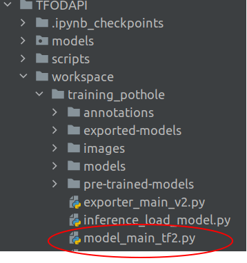
We are all set to start the training of our model. To start the training, you can change directory to the training_pothole folder and enter the following command on the terminal.

python model_main_tf2.py --model_dir=models/my_ssd_resnet50_v1_fpn --pipeline_config_path=models/my_ssd_resnet50_v1_fpn/pipeline.config

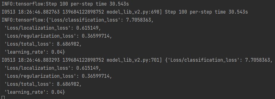
Training is a time consuming process. Depending on the speed of your computer it might take hours to complete. The process might seem stuck as not output would be printed for a long time. However you need to be patient and wait for it to complete. The metrics will be printed every 100 steps, as shown in the output above.

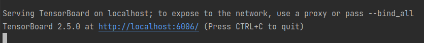
You will be able to monitor the training process using Tensorboard. You need to open a terminal, change directory to training_pothole and then enter the following command in the terminal

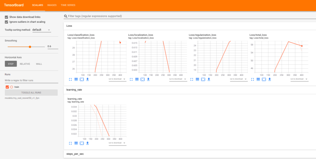
You will get the following output and tensorboard will be active on port 6006

Once you click on the link for the port 6006, you will see metrics like the below on tensorboard.

Once training is complete you will find a sessions folder called train and the checkpoints created inside my_ssd folder.

We now need to export the trained models for the inference process. This means that the model object is exported from the latest checkpoint to a new folder from which we will do our predictions.

To get this done, we first need to copy the file, TFODAPI/models/research/object_detection/exporter_main_v2.py and then paste it inside the training_pothole folder.

Now open a terminal change directory into training_pothole, directory and then enter the following command.

 python exporter_main_v2.py --input_type image_tensor --pipeline_config_path models/my_ssd_resnet50_v1_fpn/pipeline.config --trained_checkpoint_dir models/my_ssd_resnet50_v1_fpn/ --output_directory exported-models/my_model

You will now see the model object and the checkpoint information in the exported-models/my_model folder.

We can now initiate the inference process after this.

Inference Process

Inference process is where we test the model on new images. We will implement the inference process using a new script. The code for the inference step is heavily inspired from the following link

Open your text editor, create an new file and name it inference_load_model.py and add the following code into it.

import time
from object_detection.utils import label_map_util
from object_detection.utils import config_util
from object_detection.utils import visualization_utils as viz_utils
from object_detection.builders import model_builder
import os
os.environ['TF_CPP_MIN_LOG_LEVEL'] = '2'    # Suppress TensorFlow logging (1)
import tensorflow as tf
import numpy as np
from PIL import Image
import warnings
warnings.filterwarnings('ignore')   # Suppress Matplotlib warnings
import glob

First we import all the necessary packages. Packages from lines 2-5, are downloaded from the API code we downloaded. These will be available in the object detection folder.

Next we will define some of the paths to the exported model folder.

# Define the path to the model directory
PATH_TO_MODEL_DIR = "exported-models/my_model"
PATH_TO_CFG = PATH_TO_MODEL_DIR + "/pipeline.config"
PATH_TO_CKPT = PATH_TO_MODEL_DIR + "/checkpoint"

Lines 16-18, we define the paths to the model we exported, the config file and the model checkpoint. These information will be used to load the model for predictions.

We will now load the model using the check point information.

print('Loading model... ', end='')
start_time = time.time()

# Load pipeline config and build a detection model
configs = config_util.get_configs_from_pipeline_file(PATH_TO_CFG)
model_config = configs['model']
detection_model = model_builder.build(model_config=model_config, is_training=False)

# Restore checkpoint
ckpt = tf.compat.v2.train.Checkpoint(model=detection_model)
ckpt.restore(os.path.join(PATH_TO_CKPT, 'ckpt-0')).expect_partial()

end_time = time.time()
elapsed_time = end_time - start_time
print('Done! Took {} seconds'.format(elapsed_time))

We load the model in line 26 and restore the checkpoint information in lines 29-30.

Next we will see two utility functions which will be used in the inference cycle.

@tf.function
def detect_fn(image):
    """Detect objects in image."""
    image, shapes = detection_model.preprocess(image)
    prediction_dict = detection_model.predict(image, shapes)
    detections = detection_model.postprocess(prediction_dict, shapes)

    return detections

def load_image_into_numpy_array(path):
    """Load an image from file into a numpy array. """
    return np.array(Image.open(path))

The first function is to generate the detections from the image. Line 39, the image is preprocessed and we do the prediction in line 40 to get the prediction dictionary. The prediction dictionary consists of different elements which are required to create the bounding boxes for the objects. In line 41, the prediction dictionary is preprocessed to get the final detection dictionary which again consists of the elements required for bounding box creation.

The second function in lines 45-47 is a simple one to convert the image into an np.array.

Next we will initialise the labels and also get the path of the test images in lines 49-53

# Get the annotations
PATH_TO_LABELS = "annotations/label_map.pbtxt"
category_index = label_map_util.create_category_index_from_labelmap(PATH_TO_LABELS,use_display_name=True)
# Get the paths of the images
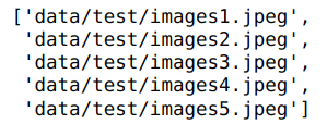
IMAGE_PATHS = glob.glob("BayesianQuest/Pothole/data/test" + '/*.jpeg')

We now have all the components to start the inference process. We will iterate through each of the test images and then create the bounding boxes. Let us see the complete process for that now.

for image_path in IMAGE_PATHS:
    print('Running inference for {}... '.format(image_path), end='')
    # Convert image into a np array
    image_np = load_image_into_numpy_array(image_path)
    # Convert the image array to a tensor after expanding the dimension to include batch size also    
    input_tensor = tf.convert_to_tensor(np.expand_dims(image_np, 0), dtype=tf.float32)
    # Get the detection
    detections = detect_fn(input_tensor)    
    # Get all the objects which were detected
    num_detections = int(detections.pop('num_detections'))
    detections = {key: value[0, :num_detections].numpy()
                  for key, value in detections.items()}
    detections['num_detections'] = num_detections
    # detection_classes should be ints.
    detections['detection_classes'] = detections['detection_classes'].astype(np.int64)
    # Create offset for labels for visualisation
    label_id_offset = 1
    image_np_with_detections = image_np.copy()
    # Visualise the images along with the bounding boxes and labels
    viz_utils.visualize_boxes_and_labels_on_image_array(
            image_np_with_detections,
            detections['detection_boxes'],
            detections['detection_classes']+label_id_offset,
            detections['detection_scores'],
            category_index,
            use_normalized_coordinates=True,
            max_boxes_to_draw=200,
            min_score_thresh=.45,
            agnostic_mode=False)
    # Show the images with bounding boxes
    img = Image.fromarray(image_np_with_detections, 'RGB')
    img.show()    

We iterate through each of the test images in line 55 and then get the detections in line 62 after all the necessary pre-processing in the previous lines.

In the pipeline.config file we defined that the maximum total objects to be 100 ( line 104 of pipeline.config file). Therefore all the elements in the detection dictionary will cater to 100 objects. However the total objects we detected could be far less that what was initialised. So for the next processes, we only need to take those objects which were detected by the model. Lines 64-69, implements the steps for selecting only those objects which were detected.

Once we get only the objects which were detected, its time to visualise the objects along with the bounding boxes and the labels. These steps are implemented in lines 71-86. In line 82, we are specifying a threshold for accepting any objects. Only those objects whose score is greater than the threshold will be visualised.

To implement the script, open the terminal and enter the following command

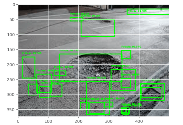
You should see outputs similar to the below after this script is run.

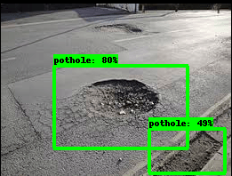
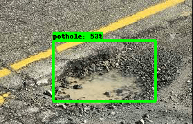
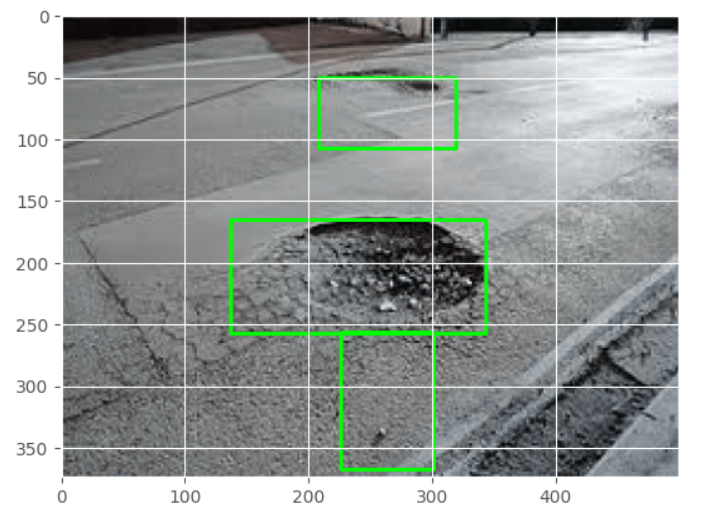
We can see that the there are some good localisations for the potholes. All these were achieved with very limited images. With more images and better pre-processing techniques, we will be able to get much better results from what we have got now.

What Next ?

So far in this series we have seen different frameworks for object detection. We started with legacy methods like image pyramids and then explored more robust methods like RCNN and YOLO. Finally in this post, we learned to implement object detection using a great utility, Tensorflow Object Detection API. Now we will move ahead from what we have learned so far. The next step is to apply the techniques we learned in some real world scenarios like using it to analyze video files. That will be our endeavor in the next post. To be notified of the next post please subscribe to this blog post .You can also subscribe to our Youtube channel for all the videos related to this series.

You can also access the code base for this series from the following git hub link

Do you want to Climb the Machine Learning Knowledge Pyramid ?

Knowledge acquisition is such a liberating experience. The more you invest in your knowledge enhacement, the more empowered you become. The best way to acquire knowledge is by practical application or learn by doing. If you are inspired by the prospect of being empowerd by practical knowledge in Machine learning, subscribe to our Youtube channel

I would also recommend two books I have co-authored. The first one is specialised in deep learning with practical hands on exercises and interactive video and audio aids for learning

This book is accessible using the following links

The Deep Learning Workshop on Amazon

The Deep Learning Workshop on Packt

The second book equips you with practical machine learning skill sets. The pedagogy is through practical interactive exercises and activities.

The Data Science Workshop Book

This book can be accessed using the following links

The Data Science Workshop on Amazon

The Data Science Workshop on Packt

Enjoy your learning experience and be empowered !!!!

Build you computer vision application IV : Building the pothole detector using RCNN

This is the fourth post of the series were we build a pothole detection application. We will be using multiple methods on computer vision which includes annotating images using labelImg, learning about object detection and localisation, mastering Tensorflow object detection API, Training objection detection using transfer learning, Object detection on video etc. This series will be split across 8 posts.

1. Introduction to object detection

2. Data set preperation and annotation Using labelImg

3. Building your object detection model from scratch using Image pyramids and sliding window

4. Building your road pothole detector using RCNN ( This Post )

5. Building your road pothole detector using YOLO

6. Building you road pothole detector using Tensorflow object detection API

7. Building your video analytics application for detecting potholes

8. Deploying your video analytics application for detection of potholes

In the last post we built an object detector from scratch using image pyramids and sliding window techniques. These techniques are legacy techniques, however important, as these techniques lay the foundation to some of the advanced techniques. In this post we will make our foray into an advanced technique by learning about the RCNN family and then will implement an object detector using RCNN. Let us dive in.

RCNN family of object detectors

RCNN framework was originally introduced by Girshik et al. in 2013. There have been several modifications to the original architecture, resulting in better performance over time. For some time the RCNN framework was the go to model for object detection tasks.

Image Source : https://arxiv.org/pdf/1311.2524.pdf

The original RCNN algorithm contains the following key steps

  • Extract regions which potentially contain an object from the input image. Such extractions are called region proposal extractions. The extractions are done using an algorithm like selective search.
  • Use a pretrained CNN to extract features from the proposal regions.
  • Classify each extracted region, using a classifier like Support Vector Machines ( SVM).

The original RCNN algorithm gave much better results than traditional methods like the sliding window and pyramid based methods. However this system was slow. Besides, deep learning was not used for localising the objects in the image and it was mostly left to algorithms like selective search.

A significant improvement was made to the original RCNN algorithm, by the same author, within a year of publishing the original paper. This algorithm was named Fast-RCNN. In this algorithm there were some novel ideas like Region of Interest Pooling layer. The Fast-RCNN algorithm used a CNN for the entire image to extract feature map from it. The region proposals were done on the feature maps extracted from the CNN layer and like the RCNN, this algorithm also used selective search for Region Proposal. A fixed size window from the feature map was extracted and then passed to a fully connected layer to get the output label for the proposal regions. This step was termed as the Region of Interest Pooling. Two sets of fully connected layers were used to get class labels of the regions along with the location of the bounding boxes for each region.

Within couple of months from the publishing of the Fast-RCNN algorithm another algorithm called the Faster-RCNN was published which improved upon the Fast-RCNN algorithm.

The new algorithm had another salient feature called the Region Proposal Network ( RPN), which was introduced to eliminate the need of selective search algorithm and build the capability for region proposal into the R-CNN architecture itself. In this algorithm, anchors were placed uniformly accross the entire image at varying scale and aspect ratios.

The image is split into equally spaced points called the anchor points and at each of the anchor point, 9 different anchors are generated and the Intersection over Union ( IOU ) of the anchors with the ground truth bounding boxes is determined to generate an objectness score. The objectness score is an indicator as to whether there is an object or not.

The objectness score is also used to filter down the number of proposals which will thereby be propogated to the subsequent binary classification and bounding box regression layer.

The binary classifier classifies the proposals as foreground ( containing an object) and background ( no object) and the regressor outputs the delta or adjustments that needs to be made to the reference anchor box, to make it similar to the ground truth bounding boxes. After these two steps in the RPN layer, the proposals are sorted based on the probability score as to whether it is foreground and background and then it undergoes Non maxima suppression to reduce the overlapping bounding boxes.

The reduced number of bounding boxes are then propogated to an ROI pooling layer which reduces the dimensions and then goes through the fully connected layers to the final softmax layers and the regressor layers. The softmax layer detects what type of object it is ( whether it is a pothole or vegetation or sign board etc) and the regressor layer gives the adjusted bounding boxes to that object.

One of the biggest advantages Faster RCNN has achieved over the previous versions is that all the moving parts can be integrated as one single network along with considerable speed in its implementation. We will leave the implementation of Faster RCNN to the subsequent chapter, where you could implement it using Tensorflow object detection API.

Having got an overview of the RCNN family, let us get to the implementation of the RCNN network.

Implementation of pothole object detector using RCNN

Let us quickly get an overview of the steps involved in the implementation of the object detector using RCNN

  1. Creation of data sets with both positive and negative images. For creation of the data sets, we will be using the image annotation details we created in post 2. We will be using the same csv file which we created in post 2.
  2. Use transfer learning technique to build our classifier. The pre-trained model we will be using is the MobileNetV2
  3. Fine tune the pre-trained model as the classifier and save the model
  4. Perform selective search algorithm using opencv for generating regions of proposals
  5. Classify the proposal regions using the fine tuned Image net model
  6. Perform non maxima suppression on the proposal regions

Let us start by importing the packages we require for this implementation

import os
import glob
import pandas as pd
import io
import cv2
import h5py
import numpy as np

from tensorflow.keras.preprocessing.image import ImageDataGenerator
from tensorflow.keras.applications import MobileNetV2
from tensorflow.keras.layers import AveragePooling2D
from tensorflow.keras.layers import Dropout
from tensorflow.keras.layers import Flatten
from tensorflow.keras.layers import Dense
from tensorflow.keras.layers import Input
from tensorflow.keras.models import Model
from tensorflow.keras.optimizers import Adam
from tensorflow.keras.applications.mobilenet_v2 import preprocess_input
from tensorflow.keras.preprocessing.image import img_to_array
from tensorflow.keras.preprocessing.image import load_img
from tensorflow.keras.utils import to_categorical
from tensorflow.keras.models import load_model
from sklearn.preprocessing import LabelBinarizer
from sklearn.model_selection import train_test_split
from sklearn.metrics import classification_report
from sklearn.feature_extraction.image import extract_patches_2d
from imutils import paths
import matplotlib.pyplot as plt
import pickle
import imutils

Data Preprocessing

For data preprocessing we have to convert the data and labels into arrays for us to train our models. We have two classes of data i.e the positive class which pertains to the potholes and the negative class which are those images other than potholes. We have to preprocess both these images seperately.

Let us start the process with the positive class. We will be using the ‘csv’ file which we created in Post 2 for getting the required information on the positive classes. Let us read the csv files and create two empty lists to store the data and labels.

# Reading the csv file
pothole_df = pd.read_csv('pothole_df.csv')

Let us explore the head of the positive class information data frame

pothole_df.head()
figure 1 : Positive class information

Each row of the data frame contains information on the file name of our image along with the localisation information of the pothole. We will be using these information to extract the region of interest ( roi ) from the image. Let us now get to creating the roi’s from this information. To start off we will create two empty lists to store the roi features and the labels.

# Empty lists to store data and labels
data = []
labels = []

Next we will create a function to extract the region of interest(roi’s) from the positive class. This class is similar to the one which we created in the previous post.

Region of interest Extractor for positive and negative classes

# Functions to extract the bounding boxes and preprocess the image
def roiExtractor(row,path):
    img = cv2.imread(path + row['filename'])    
    # Get the bounding box elements
    bb = [int(row['xmin']),int(row['ymin']),int(row['xmax']),int(row['ymax'])]
    # Crop the image
    roi = img[bb[1]:bb[3], bb[0]:bb[2]]
    # Reshape the image
    roi = cv2.resize(roi,(224,224),interpolation=cv2.INTER_CUBIC)    
    # Convert the image to an array
    roi = img_to_array(roi)
    # Preprocess the image
    roi = preprocess_input(roi)    
    return roi

The inputs to the function are each row of the csv file and the path to the folder where the images are placed. We first read the image in line 39.The image is read by concatenating the path to the images folder and the filename listed in the csv file. Once the image is read, the bounding box information for the image is extracted in line 41 and then the image is cropped to get only the positive classes in line 43. The images are then resized to a standard size of (224,224 )in line 45. We resize it to a standard dimension as that is the dimension required for the Mobilenet network. In lines 47-49, the images are converted to arrays and then preprocessed. The preprocess_input() method in line 49 normalises the pixel values so that it is between 0-1.

We will process the images based on the function we just created. We iterate through each row of the csv file ( line 54) and then extract only those rows where the class is ‘pothole’ ( line 55). We get the roi using the roiExtractor function ( line 56) and then append the roi to the list we created (data) ( line 58). The labels for the positive class are also appended to labels ( line 59) .

# This is the path where the images are placed. Change this path to the location you have defined
path = 'data/'
# Looping through the excel sheet rows
for idx, row in pothole_df.iterrows():    
    if row['class'] == 'pothole':
        roi = roiExtractor(row,path)
        # Append the data and labels for the positive class
        data.append(roi)
        labels.append(int(1))
print(len(data))
print(data[0].shape)

I have 31 roi’s of the positive class with a shape of (224,224,3).

Having processed the positive examples, let us now extract the negative examples. As seen in the previous post the negative classes are general images of roads without potholes.

# Listing all the negative examples
path = 'data/Annotated'
roadFiles = glob.glob(path + '/*.jpeg')
print(len(roadFiles))

I have selected 21 negative examples. You are free to get as many of these examples as possible. Only point which should be ensured is that there should be a good balance between the positive and negative class. We will now process the negative class images

# Looping through the images of negative class
for row in roadFiles:
    # Read the image
    img = cv2.imread(row)
    # Extract patches
    patches = extract_patches_2d(img,(128,128),max_patches=2)
    # For each patch do the augmentation
    for patch in patches:        
        # Reshape the image
        roi = cv2.resize(patch,(224,224),interpolation=cv2.INTER_CUBIC)
        #print(roi.shape)
        # Convert the image to an array
        roi = img_to_array(roi)
        # Preprocess the image
        roi = preprocess_input(roi)
        #print(roi.shape)
        # Append the data into the data folder and labels folder
        data.append(roi)
        labels.append(int(0))    

For the negative classes, we iterate through each of the images and then read them in line 69. We then extract two patches each of size (128,128) from the image in line 71. Each patch is then resized to the standard size and the converted to array and preprocessed in lines 75-80. Finally the patches are appended to data and labels are appended as ‘0’.

Let us now take a count of the total examples we have

print(len(data))

We now have 73 examples which comprises of 31 positive classes and 42 ( 21 x 2 patches each ) negative classes.

Preparing the train and test sets

We will now convert the data and labels into arrays and then perform one hot encoding to the labels for preperation of our train and test sets.

# convert the data and labels to NumPy arrays
data = np.array(data, dtype="float32")
labels = np.array(labels)
print(data.shape)
print(labels.shape)
# perform one-hot encoding on the labels
lb = LabelBinarizer()
# Fit transform the labels array
labels = lb.fit_transform(labels)
# Convert this to categorical 
labels = to_categorical(labels)
print(labels.shape)
labels

After one hot encoding the labels array is transformed into a shape (73,2), where the second dimension is the class label. The first class is our negative class [0] and the second one is the positive class [1].

Finally let us create our train and test sets using a 85:15 split. We are taking a higher proportion of train set since we have very less training examples.

# Partition data to train and test set with 85 : 15 split
(trainX, testX, trainY, testY) = train_test_split(data, labels,test_size=0.15, stratify=labels, random_state=42)
print("training data shape :",trainX.shape)
print("testing data shape :",testX.shape)
print("training labels shape :",trainY.shape)
print("testing labels shape :",testY.shape)

Now that we have finished the data processing its time to start our training process

Training a MobilenetV2 model using transfer learning : Warming up phase

We will be building our object detector model using transfer learning process. To build our transfer learned model for pothole detection we will be using MobileNetV2 as our base network. We will remove the top layer and then build our custom layer to cater to our use case. Let us see how we build our network.

# Create the base network by removing the top of the MobileNetV2 model
baseNetwork = MobileNetV2(weights="imagenet", include_top=False,input_tensor=Input(shape=(224, 224, 3)))
# Create a custom head network on top of the basenetwork to cater to two classes.
topNetwork = baseNetwork.output
topNetwork = AveragePooling2D(pool_size=(5, 5))(topNetwork)
topNetwork = Flatten(name="flatten")(topNetwork)
topNetwork = Dense(128, activation="relu")(topNetwork)
topNetwork = Dropout(0.5)(topNetwork)
topNetwork = Dense(2, activation="softmax")(topNetwork)
# Place our custom top layer on top of the base layer. We will only train the base layer.
model = Model(inputs=baseNetwork.input, outputs=topNetwork)
# Freeze the base network so that they are not updated during the training process
for layer in baseNetwork.layers:
    layer.trainable = False

We load the base network in line 106. The base network is the MobileNetV2 and we exclude the top layer by specifying the parameter , include_top=False. We also specify the shape of the input layer.

Its now time to specify our custom network. We build our custom network on top of the output of the base network as shown in line 108. From lines 109-112, we build the different layers of our custom layer starting with the AveragePooling layer and the final Dense layer. In line 113 we define the final Softmax layer for our 2 classes. We then define the model using the Model() class with the inputs as the baseNetwork input and the output as the custom network we have defined in line 115.

In line 117, we specify which layers needs to be trained. Here we are specifying that the base network layers need not be trained. This is because the base network is already pre-trained and our custom layer is the one which is not trained. By specifying that only our custom layer be trained ( or alternatively the base network need not be trained), we are optimising the custom layer. This process can be called the warming up process for the custom layer. Once the custom layer is warmed up after some iterations, we can even specify that some layers of the base network too can be trained. We will perform all these steps.

First let us train our custom layer. We start off the process by defining our training parameters like learning rate, number of epochs and the batch size.

# Initialise the learning rate, epochs and batch size
LR = 1e-4
epoc = 5
bs = 16

You might be surprise that the epochs we have selecte is only 5. This is because since the base network is pre-trained we dont have to train the custom layer for many epochs. Besides we are only warming up the custom layer.

Next let us define the data generator along with the augmentation layer.

# Create a image generator with data augmentation
aug = ImageDataGenerator(rotation_range=40,zoom_range=0.25,width_shift_range=0.2,height_shift_range=0.2,shear_range=0.30,
 horizontal_flip=True,fill_mode="nearest")

In the previous post we implemented manual data augmentation methods. Keras has a great method to do image augmentation during training using the ImageDataGenerator(). It lets us do all the augmentation we did manually in the previous post.

We have now defined most of the moving parts required for training. Lets now define the optimiser and then compile the model and then fit the model with the data set.

# Compile the model
print("[INFO] compiling model...")
opt = Adam(lr=LR)
model.compile(loss="binary_crossentropy", optimizer=opt,metrics=["accuracy"])
# Training the customer head network
print("[INFO] training the model...")
history = model.fit(aug.flow(trainX, trainY, batch_size=bs),steps_per_epoch=len(trainX) // bs,validation_data=(testX, testY),
 validation_steps=len(testX) // bs,epochs=epoc)

Training some layers of the base network

We have done the warm up of the custom head we placed over the base network. Now let us also train some of the layers of the network along with the head. Let us first print out all the layers of the base network to determine the layers we want to train along with our head.

for (i,layer) in enumerate(baseNetwork.layers):
    print(" [INFO] {}\t{}".format(i,layer.__class__.__name__))

In line 134, we iterate through each of the layers of the base network and the print the name of the layer.

We can see that there are 153 layers in the base network. Let us train from layer 140 onwards and freeze all the layers above 140.

for layer in baseNetwork.layers[140:]:
    layer.trainable = True

# Compile the model
print("[INFO] Compiling the model again...")
opt = Adam(lr=LR)
model.compile(loss="binary_crossentropy", optimizer=opt,metrics=["accuracy"])
# Training the customer head network
print("[INFO] Fine tuning the model along with some layers of base network...")
history = model.fit(aug.flow(trainX, trainY, batch_size=bs),steps_per_epoch=len(trainX) // bs,validation_data=(testX, testY),
 validation_steps=len(testX) // bs,epochs=epoc)

With the new training we can see that the accuracy has jumped to 98% from the initial 80%. Let us predict on test set and then print the classification report.

For generating the classification report let us convert the label names into a string as shown below

# Converting the target names as string for classification report
target_names = list(map(str,lb.classes_))

Let us now print the classification report and see how well our model is performing on the test set

# make predictions on the test set
print("[INFO] Generating inference...")
predictions = model.predict(testX, batch_size=bs)
# For each prediction we need to find the index with maximum probability 
predIdxs = np.argmax(predictions, axis=1)
# Print the classification report
print(classification_report(testY.argmax(axis=1), predIdxs,target_names=target_names))

We get the predictions which are in the form of probabilities for each class in line 151. We then extract the id of the class which has the maximum probability using the np.argmax method in line 153. Finally we generate the classification report in line 155. We can see that we have a near perfect classification report as shown below.

Let us also visualise our training accuracy and loss and then save the figure.

# plot the training loss and accuracy
N = epoc
plt.style.use("ggplot")
plt.figure()
plt.plot(np.arange(0, N), history.history["loss"], label="train_loss")
plt.plot(np.arange(0, N), history.history["accuracy"], label="train_acc")
plt.title("Training Loss and Accuracy")
plt.xlabel("Epoch #")
plt.ylabel("Loss/Accuracy")
plt.legend(loc="lower left")
plt.savefig("plot.png")
plt.show()

Let us finally save our model and the label binarizer so that we can use it later in our inference process

MODEL_PATH = "output/pothole_detector_RCNN.h5"
ENCODER_PATH = "output/label_encoder_RCNN.pickle"
# serialize the model to disk
print("[INFO] saving pothole detector model...")
model.save(MODEL_PATH, save_format="h5")
# serialize the label encoder to disk
print("[INFO] saving label encoder...")
f = open(ENCODER_PATH, "wb")
f.write(pickle.dumps(lb))
f.close()

We have completed the training cycle and have saved the model. Let us now implement the inference cycle.

Inference run for pothole detection

In the inference cycle, we will use the model we just built to localise and predict potholes in test images. Let us first load the model and the label encoder which we saved.

MODEL_PATH = "output/pothole_detector_RCNN.h5"
ENCODER_PATH = "output/label_encoder_RCNN.pickle"
print("[INFO] loading model and label binarizer...")
model = load_model(MODEL_PATH)
lb = pickle.loads(open(ENCODER_PATH, "rb").read())

We have downloaded some test files. Lets visualise some of them here

# Please change the path where your files are placed
testpath = 'data/test'
testFiles = glob.glob(testpath + '/*.jpeg')
testFiles

Lets plot one of the images

# load the input image from disk
image = cv2.imread(testFiles[2])
#Resize the image and plot the image
image = imutils.resize(image, width=500)
plt.imshow(image,aspect='equal')
plt.show()

We will use Opencv to generate the bounding boxes proposals for the image. Detailed below are the specific steps for the selective search implementation using Opencv to generate the bounding boxes. The set of proposals would be contained in the variable rects

# Implementing selective search to generate bounding box proposals
print("[INFO] running selective search and generating bounding boxes...")
ss = cv2.ximgproc.segmentation.createSelectiveSearchSegmentation()
ss.setBaseImage(image)
ss.switchToSelectiveSearchFast()
rects = ss.process()

Let us look how many proposals the selective search algorithm has generated

len(rects)

For this specific image as you can see the selective search algorithm has generated 920 proposals. As you know these are regions where there is high probability to find an object. As you might have noticed this specific algorithm is pretty slow in identifying all the bounding boxes.

Next let us extract the region of interest from the image using the bounding boxes we obtained from the selective search algorithm. Let us explore the code

# Initialise lists to store the region of interest from the image and its bounding boxes
proposals = []
boxes = []
max_proposals = 100
# Iterate over the bounding box coordinates to extract region of interest from image
for (x, y, w, h) in rects[:max_proposals]:    
    # Crop region of interest from the image
	roi = image[y:y + h, x:x + w]
    # Convert to RGB format as CV2 has output in BGR format
	roi = cv2.cvtColor(roi, cv2.COLOR_BGR2RGB)
    # Resize image to our standar size
	roi = cv2.resize(roi, (224,224),
		interpolation=cv2.INTER_CUBIC)
	# Preprocess the image
	roi = img_to_array(roi)
	roi = preprocess_input(roi)
	# Update the proposal and bounding boxes
	proposals.append(roi)
	boxes.append((x, y, x + w, y + h))

In lines 200-201, we initialise two lists for storing the roi’s and their bounding box co-oridinates. In line 202, we also define the max number of proposals we want. This step is to improve the speed of computation by eliminating processing of too many proposals. This is a parameter you can vary and I would encourage you to try out different values for this parameter.

Next we iterate through each of the bounding boxes we want, to extract the region of interest and their bounding boxes as detailed in lines 205-215. The various processes we implement are to crop the images, covert the images to RGB format, resize to the desired size and the final normalization of the pixel values. Finally the roi and bounding boxes are updated in lines 217-218 to the lists we created earlier.

Its now time to classify the regions of proposal using the model we fine tuned. Before classification we have to convert the lists to a numpy array. Let us implement these processes.

# Convert proposals and bouding boxes to NumPy arrays
proposals = np.array(proposals, dtype="float32")
boxes = np.array(boxes, dtype="int32")
print("[INFO] proposal shape: {}".format(proposals.shape))
# Classify the proposals based on the fine tuned model
print("[INFO] classifying proposals...")
proba = model.predict(proposals)

Next we will extract those roi’s which are classified as ‘potholes’ from the overall predictions.

# Find the predicted labels 
labels = lb.classes_[np.argmax(proba, axis=1)]
# Get the ids where the predictions are 'Potholes'
idxs = np.where(labels == 1)[0]
idxs

The model prediction gives us the probability of each class. We will find the predicted labels from the probability by taking the argmax of the predicted class probabilities as shown in line 227. Once we have the labels, we extract the indexes of the pothole class in line 229, which in our case is 1.

Next using the indexes we will extract the bounding boxes and probability of the ‘pothole’ class

# Using the indexes, extract the bounding boxes and prediction probabilities of 'pothole' class
boxes = boxes[idxs]
proba = proba[idxs][:, 1]

Next we will apply another filter and take only those bounding boxes which has a probability greater than a threshold value.

print(len(boxes))
# Filter the bounding boxes using a prediction probability threshold
pred_threshold = 0.995
# Select only those ids where the probability is greater than the threshold
idxs = np.where(proba >= pred_threshold)
boxes = boxes[idxs]
proba = proba[idxs]
print(len(boxes))

The threshold has been fixed in this case by experimenting with different values. This is another hyperparameter which needs to be arrived at observing the predictions you obtain for your specific set of images. We can see that before filtering we had 97 bounding boxes which has got reduced to 22 after the filtering. These filtered bounding boxes will be used to localise potholes on the image. Let us visualise the filtered bounding boxes on the image.

# Clone the original image for visualisation and inserting text
clone = image.copy()
# Iterate through the bounding boxes and associated probabilities
for (box, prob) in zip(boxes, proba):
    # Draw the bounding box, label, and probability on the image
    (startX, startY, endX, endY) = box
    cv2.rectangle(clone, (startX, startY), (endX, endY),(0, 255, 0), 2)
    # Initialising the cordinate for writing the text
    y = startY - 10 if startY - 10 > 10 else startY + 10
    # Getting the text to be attached on top of the box
    text= "Pothole: {:.2f}%".format(prob * 100)
    # Visualise the text on the image
    cv2.putText(clone, text, (startX, y),cv2.FONT_HERSHEY_SIMPLEX, 0.25, (0, 255, 0), 1)
# Visualise the bounding boxes on the image
plt.imshow(clone,aspect='equal')
plt.show() 

We clone the image in line 243 and then iterate through the boxes in lines 245 – 254. When we iterate through each box and grab the co-ordinates in line 247 and first draw the rectangle over the image with those co-ordinates in line 248. In the subsequent lines we print the class name and also the probability of the class on top of the bounding box. Finally we visualise the image with the bounding boxes and the text in lines 256-257.

As we can see we have the bounding boxes over the potholes and also regions around them also. However we can see that we have multiple overlapping boxes which ultimately needs to be reduced. So our next task is to apply non maxima suppression to reduce the number of bounding boxes.

Non Maxima Suppression

We will use the same method we used in the previous post for the non maxima suppression. Let us get the function for non maxima suppression. For explanation on this function please refer the previous post

def maxOverlap(boxes):
    '''
    boxes : This is the cordinates of the boxes which have the object
    returns : A list of boxes which do not have much overlap
    '''
    # Convert the bounding boxes into an array
    boxes = np.array(boxes)
    # Initialise a box to pick the ids of the selected boxes and include the largest box
    selected = []
    # Continue the loop till the number of ids remaining in the box is greater than 1
    while len(boxes) > 1:
        # First calculate the area of the bounding boxes 
        x1 = boxes[:, 0]
        y1 = boxes[:, 1]
        x2 = boxes[:, 2]
        y2 = boxes[:, 3]
        area = (x2 - x1) * (y2 - y1)
        # Sort the bounding boxes based on its area    
        ids = np.argsort(area)
        #print('ids',ids)
        # Take the coordinates of the box with the largest area
        lx1 = boxes[ids[-1], 0]
        ly1 = boxes[ids[-1], 1]
        lx2 = boxes[ids[-1], 2]
        ly2 = boxes[ids[-1], 3]
        # Include the largest box into the selected list
        selected.append(boxes[ids[-1]].tolist())
        # Initialise a list for getting those ids that needs to be removed.
        remove = []
        remove.append(ids[-1])
        # We loop through each of the other boxes and find the overlap of the boxes with the largest box
        for id in ids[:-1]:
            #print('id',id)
            # The maximum of the starting x cordinate is where the overlap along width starts
            ox1 = np.maximum(lx1, boxes[id,0])
            # The maximum of the starting y cordinate is where the overlap along height starts
            oy1 = np.maximum(ly1, boxes[id,1])
            # The minimum of the ending x cordinate is where the overlap along width ends
            ox2 = np.minimum(lx2, boxes[id,2])
            # The minimum of the ending y cordinate is where the overlap along height ends
            oy2 = np.minimum(ly2, boxes[id,3])
            # Find area of the overlapping coordinates
            oa = (ox2 - ox1) * (oy2 - oy1)
            # Find the ratio of overlapping area of the smaller box with respect to its original area
            olRatio = oa/area[id]            
            # If the overlap is greater than threshold include the id in the remove list
            if olRatio > 0.40:
                remove.append(id)                
        # Remove those ids from the original boxes
        boxes = np.delete(boxes, remove,axis = 0)
        # Break the while loop if nothing to remove
        if len(remove) == 0:
            break
    # Append the remaining boxes to the selected
    for i in range(len(boxes)):
        selected.append(boxes[i].tolist())
    return np.array(selected)

Let us now apply the non maxima suppression function and eliminate the overlapping boxes.

# Applying non maxima suppression
selected = maxOverlap(boxes)
len(selected)

We can see that by applying non maxima suppression we have reduced the number of boxes from 22 to around 3. Let us now visualise the images with the selected list of bounding boxes after non maxima suppression.

clone = image.copy()
plt.imshow(image,aspect='equal')
for (startX, startY, endX, endY) in selected:
    cv2.rectangle(clone, (startX, startY), (endX, endY), (0, 255, 0), 2)       

plt.imshow(clone,aspect='equal')
plt.show()

We can see that the number of bounding boxes have considerably reduced and have localised well to the two potholes.

With this we have come to the end of object detection using RCNN. Let us quickly recap what we have achieved in this post.

  1. We preprocessed the positive and negative classes of images and then built our train and test sets
  2. Fine tuned the MobileNet model to cater to our use case and made it our classifier.
  3. Built the inference pipeline using the fine tuned classifier
  4. Applied non maxima suppression to get the bounding boxes over the potholes.

We have come a long way and are now adept at implementing an advanced model like RCNN. However there are still variations to this model which we could try. One of the variations we can try is to implement a RCNN for multiple classes. So lets say we predict potholes and also road signs with the same network. Implementing a multiclass RCNN would adopt the same processes with a little variation during the model architecture and training. We will build a multiclass RCNN framework in a future post.

What Next ?

Having seen an advanced method like RCNN, we will go to another advanced method in the next post, which is Yolo. Yolo is a more faster method than RCNN and will enable us to use the road detection process in video files. We will be covering pothole detection using Yolo in the next post and then use it to detect potholes on videos in the subsequent post. Watch this space for more.

To be notified of the next post please subscribe to this blog post .You can also subscribe to our Youtube channel for all the videos related to this series.

You can also access the code base for this series from the following git hub link

Do you want to Climb the Machine Learning Knowledge Pyramid ?

Knowledge acquisition is such a liberating experience. The more you invest in your knowledge enhacement, the more empowered you become. The best way to acquire knowledge is by practical application or learn by doing. If you are inspired by the prospect of being empowerd by practical knowledge in Machine learning, subscribe to our Youtube channel

I would also recommend two books I have co-authored. The first one is specialised in deep learning with practical hands on exercises and interactive video and audio aids for learning

This book is accessible using the following links

The Deep Learning Workshop on Amazon

The Deep Learning Workshop on Packt

The second book equips you with practical machine learning skill sets. The pedagogy is through practical interactive exercises and activities.

The Data Science Workshop Book

This book can be accessed using the following links

The Data Science Workshop on Amazon

The Data Science Workshop on Packt

Enjoy your learning experience and be empowered !!!!

Building Self Learning Recommendation system – VIII : Evaluating deployment options

This is the eighth and last post of our series on building a self learning recommendation system using reinforcement learning. This series consists of 8 posts where in we progressively build a self learning recommendation system.

  1. Recommendation system and reinforcement learning primer
  2. Introduction to multi armed bandit problem
  3. Self learning recommendation system as a K-armed bandit
  4. Build the prototype of the self learning recommendation system : Part I
  5. Build the prototype of the self learning recommendation system : Part II
  6. Productionising the self learning recommendation system : Part I – Customer Segmentation
  7. Productionising self learning recommendation system: Part II : Implementing self learning recommendations
  8. Evaluating deployment options for the self learning recommendation systems. ( This post )

This post ties together all what we discussed in the previous two posts where in we explored all the classes and methods we built for the application. In this post we will implement the driver file which controls all the processes and then explore different options to deploy this application.

Implementing the driver file

Now that we have seen all the classes and methods of the application, let us now see the main driver file which will control the whole process.

Open a new file and name it rlRecoMain.py and copy the following code into the file

import argparse
import pandas as pd
from utils import Conf,helperFunctions
from Data import DataProcessor
from processes import rfmMaker,rlLearn,rlRecomend
import os.path
from pymongo import MongoClient

# Construct the argument parser and parse the arguments
ap = argparse.ArgumentParser()
ap.add_argument('-c','--conf',required=True,help='Path to the configuration file')
args = vars(ap.parse_args())

# Load the configuration file
conf = Conf(args['conf'])

print("[INFO] loading the raw files")
dl = DataProcessor(conf)

# Check if custDetails already exists. If not create it
if os.path.exists(conf["custDetails"]):
    print("[INFO] Loading customer details from pickle file")
    # Load the data from the pickle file
    custDetails = helperFunctions.load_files(conf["custDetails"])
else:
    print("[INFO] Creating customer details from csv file")
    # Let us load the customer Details
    custDetails = dl.gvCreator()
    # Starting the RFM segmentation process
    rfm = rfmMaker(custDetails,conf)
    custDetails = rfm.segmenter()
    # Save the custDetails file as a pickle file 
    helperFunctions.save_clean_data(custDetails,conf["custDetails"])

# Starting the self learning Recommendation system

# Check if the collections exist in Mongo DB
client = MongoClient(port=27017)
db = client.rlRecomendation

# Get all the collections from MongoDB
countCol = db["rlQuantdic"]
polCol = db["rlValuedic"]
rewCol = db["rlRewarddic"]
recoCountCol = db['rlRecotrack']

print(countCol.estimated_document_count())

# If Collections do not exist then create the collections in MongoDB
if countCol.estimated_document_count() == 0:
    print("[INFO] Main dictionaries empty")
    rll = rlLearn(custDetails, conf)
    # Consolidate all the products
    rll.prodConsolidator()
    print("[INFO] completed the product consolidation phase")
    # Get all the collections from MongoDB
    countCol = db["rlQuantdic"]
    polCol = db["rlValuedic"]
    rewCol = db["rlRewarddic"]

# start the recommendation phase
rlr = rlRecomend(custDetails,conf)
# Sample a state since the state is not available
stateId = rlr.stateSample()
print(stateId)

# Get the respective dictionaries from the collections

countDic = countCol.find_one({stateId: {'$exists': True}})
polDic = polCol.find_one({stateId: {'$exists': True}})
rewDic = rewCol.find_one({stateId: {'$exists': True}})

# The count dictionaries can exist but still recommendation dictionary can not exist. So we need to take this seperately

if recoCountCol.estimated_document_count() == 0:
    print("[INFO] Recommendation tracking dictionary empty")
    recoCountdic = {}
else:
    # Get the dictionary from the collection
    recoCountdic = recoCountCol.find_one({stateId: {'$exists': True}})


print('recommendation count dic', recoCountdic)


# Initialise the Collection checker method
rlr.collfinder(stateId,countDic,polDic,rewDic,recoCountdic)
# Get the list of recommended products
seg_products = rlr.rlRecommender()
print(seg_products)
# Initiate customer actions

click_list,buy_list = rlr.custAction(seg_products)
print('click_list',click_list)
print('buy_list',buy_list)

# Get the reward functions for the customer action
rlr.rewardUpdater(seg_products,buy_list ,click_list)

We import all the necessary libraries and classes in lines 1-7.

Lines 10-12, detail the argument parser process. We provide the path to our configuration file as the argument. We discussed in detail about the configuration file in post 6 of this series. Once the path of the configuration file is passed as the argument, we read the configuration file and the load the value in the variable conf in line 15.

The first of the processes is to initialise the dataProcessor class in line 18. As you know from post 6, this class has the methods for loading and processing data. After this step, lines 21-33 implements the raw data loading and processing steps.

In line 21 we check if the processed data frame custDetails is already present in the output directory. If it is present we load it from the folder in line 24. If we havent created the custDetails data frame before, we initiate that action in line 28 using the gvCreator method we have seen earlier. In lines 30-31, we create the segments for the data using the segmenter method in the rfmMaker class. Finally the custDetails data frame is saved as a pickle file in line 33.

Once the segmentation process is complete the next step is to start the recommendation process. We first establish the connection with our collection in lines 38-39. Then we collect the 4 collections from MongoDB in lines 42-45. If the collections do not exist it will return a ‘None’.

If the collections are none, we need to create the collections. This is done in lines 50-59. We instantiate the rlLearn class in line 52 and the execute the prodConsolidator() method in line 54. Once this method is run the collections would be created. Please refer to the prodConsolidator() method in post 7 for details. Once the collections are created, we get those collections in lines 57-59.

Next we instantiate the rlRecomend class in line 62 and then sample a stateID in line 64. Please note that the sampling of state ID is only a work around to simulate a state in the absence of real customer data. If we were to have a live application, then the state Id would be created each time a customer logs into the sytem to buy products. As you know the state Id is a combination of the customers segment, month and day in which the logging happens. So as there are no live customers we are simulating the stateId for our online recommendation process.

Once we have sampled the stateId, we need to extract the dictionaries corresponding to that stateId from the MongoDb collections. We do that in lines 69-71. We extract the dictionary corresponding to the recommendation as a seperate step in lines 75-80.

Once all the dictionaries are extracted, we do the initialisation of the dictionaries in line 87 using the collfinder method we explored in post 7 . Once the dictionaries are initialised we initiate the recommendation process in line 89 to get the list of recommended products.

Once we get the recommended products we simulate customer actions in line 93, and then finally update the rewards and values using rewardUpdater method in line 98.

This takes us to the end of the complete process to build the online recommendation process. Let us now see how this application can be run on the terminal

Figure 1 : Running the application on terminal

The application can be executed on the terminal with the below command

$ python rlRecoMain.py --conf config/custprof.json

The argument we give is the path to the configuration file. Please note that we need to change directory to the rlreco directory to run this code. The output from the implementation would be as below

The data can be seen in the MongoDB collections also. Let us look at ways to find the data in MongoDB collections.

To initialise Mongo db from terminal, use the following command

Figure 3 : Initialize Mongo

You should get the following output

Now to find all the data bases in Mongo DB you can use the below command

You will be able to see all the databases which you have created. The one marked in red is the database we created. No to use that data base the command used is use rlRecomendation as shown below. We will get the command that the database has been switched to the desired data base.

To see all the collections we have made in this database we can use the below command.

From the output we can see all the collections we have created. Now to see some specific record within the collections, we can use the following command.

db.rlValuedic.find({"Q1_August_1_Monday":{$exists:true} })

In the above command we are trying to find all records in the collection rlValuedic for the stateID "Q1_August_1_Monday". Once we execute this command we get all the records in this collection for this specific stateID. You should get the below output.

The output displays all the proucts for that stateID and its value function.

What we have implemented in code is a simulation of the complete process. To run this continuously for multiple customers, we can create another scrip with a list of desired customers and then execute the code multiple times. I will leave that step as an exercise for you to implement. Now let us look at different options to deploy this application.

Deployment of application

The end product of any data science endeavour should be to build an application and sharing it with the world. There are different options to deploy python applications. Let us look at some of the options available. I would encourage you to explore more methods and share your results.

Flask application with Heroku

A great option to deploy your applications is to package it as a Flask application and then deploy it using Heroku. We have discussed this option in one of our earlier series, where we built a machine translation application. You can refer this link for details. In this section we will discuss the nuances of building the application in Flask and then deploying it on Heroku. I will leave the implementation of the steps for you as an exercise.

When deploying the self learning recommendation system we have built, the first thing which we need to design is what the front end will contain. From the perspective of the processes we have implemented, we need to have the following processes controlled using the front end.

  1. Training process : This is the process which takes the raw data, preprocesses the data and then initialises all the dictionaries. This includes all the processes till line 59 in the driver file rlRecoMain.py. We need to initialise the process of training from the front end of the flask application. In the background all the process till line 59 should run and the dictionaries needs to be updated.
  2. Recommendation simulation : The second process which needs to be controlled is the one where we get the recommendations. The start of this process is the simulation of the state from the front end. To do this we can provide a drop down of all the customer IDs on the flask front end and take the system time details to form the stateID. Once this stateID is generated, we start the recommendation process which includes all the process starting from line 62 till line 90 in the the driver file rlRecoMain.py. Please note that line 64 is the stateID simulating process which will be controlled from the front end. So that line need not be implemented. The final output, which is the list of all recommended products needs to be displayed on the front end. It will be good to add some visual images along with the product for visual impact.
  3. Customer action simulation : Once the recommended products are displayed on the front end, we can send feed back from the front end in terms of the products clicked and the products bought through some widgets created in the front end. These widgets will take the place of line 93, in our implementation. These feed back from the front end needs to be collected as lists, which will take the place of click_list and buy_list given in lines 94-95. Once the customer actions are generated, the back end process in line 98, will have to kick in to update the dictionaries. Once the cycle is completed we can build a refresh button on the screen to simulate the recommendation process again.

Once these processes are implemented using a Flask application, the application can be deployed on Heroku. This post will give you overall guide into deploying the application on Heroku.

These are broad guidelines for building the application and then deploying them. These need not be the most efficient and effective ones. I would challenge each one of you to implement much better processes for deployment. Request you to share your implementations in the comments section below.

Other options for deployment

So far we have seen one of the option to build the application using Flask and then deploy them using Heroku. There are other options too for deployment. Some of the noteable ones are the following

  • Flask application on Ubuntu server
  • Flask application on Docker

The attached link is a great resource to learn about such deployment. I would challenge all of you to deploy using any of these implementation steps and share the implementation for the community to benefit.

Wrapping up.

This is the last post of the series and we hope that this series was informative.

We will start a new series in the near future. The next series will be on a specific problem on computer vision specifically on Object detection. In the next series we will be building a ‘Road pothole detector using different object detection algorithms. This series will touch upon different methods in object detection like Image Pyramids, RCNN, Yolo, Tensorflow Object detection API etc. Watch out this space for the next series.

Please subscribe to this blog post to get notifications when the next post is published.

You can also subscribe to our Youtube channel for all the videos related to this series.

The complete code base for the series is in the Bayesian Quest Git hub repository

Do you want to Climb the Machine Learning Knowledge Pyramid ?

Knowledge acquisition is such a liberating experience. The more you invest in your knowledge enhacement, the more empowered you become. The best way to acquire knowledge is by practical application or learn by doing. If you are inspired by the prospect of being empowerd by practical knowledge in Machine learning, subscribe to our Youtube channel

I would also recommend two books I have co-authored. The first one is specialised in deep learning with practical hands on exercises and interactive video and audio aids for learning

This book is accessible using the following links

The Deep Learning Workshop on Amazon

The Deep Learning Workshop on Packt

The second book equips you with practical machine learning skill sets. The pedagogy is through practical interactive exercises and activities.

The Data Science Workshop Book

This book can be accessed using the following links

The Data Science Workshop on Amazon

The Data Science Workshop on Packt

Enjoy your learning experience and be empowered !!!!

Building Self Learning Recommendation system – VII : Productionizing the application : II

This is the seventh post of our series on building a self learning recommendation system using reinforcement learning. This series consists of 8 posts where in we progressively build a self learning recommendation system.

  1. Recommendation system and reinforcement learning primer
  2. Introduction to multi armed bandit problem
  3. Self learning recommendation system as a K-armed bandit
  4. Build the prototype of the self learning recommendation system : Part I
  5. Build the prototype of the self learning recommendation system : Part II
  6. Productionising the self learning recommendation system : Part I – Customer Segmentation
  7. Productionising the self learning recommendation system: Part II – Implementing self learning recommendation ( This Post )
  8. Evaluating different deployment options for the self learning recommendation systems.

This post builds on the previous post where we started off with productionizing the application using python scripts. In the last post we completed the customer segmentation part. In this post we continue from where we left off and then build the self learning system using python scripts. Let us get going.

Creation of States

Let us take a quick recap of the project structure and what we covered in the last post.

In the last post we were in the early part of our main driver file rlRecoMain.py. We explored rfmMaker class in file rfmProcess.py from the processes directory. We will now explore selfLearnProcess.py file in the same directory.

Open a new file and name it selfLearnProcess.py and insert the following code

import pandas as pd
from numpy.random import normal as GaussianDistribution
from collections import OrderedDict
from collections import Counter
import operator
from random import sample
import numpy as np
from pymongo import MongoClient
client = MongoClient(port=27017)
db = client.rlRecomendation


class rlLearn:
    def __init__(self,custDetails,conf):
        # Get the date  as a seperate column
        custDetails['Date'] = custDetails['Parse_date'].apply(lambda x: x.strftime("%d"))
        # Converting date to float for easy comparison
        custDetails['Date'] = custDetails['Date'].astype('float64')
        # Get the period of month column
        custDetails['monthPeriod'] = custDetails['Date'].apply(lambda x: int(x > conf['monthPer']))
        # Aggregate the custDetails to get a distribution of rewards
        rewardFull = custDetails.groupby(['Segment', 'Month', 'monthPeriod', 'Day', conf['product_id']])[conf['prod_qnty']].agg(
            'sum').reset_index()
        # Get these data frames for all methods
        self.custDetails = custDetails
        self.conf = conf
        self.rewardFull = rewardFull
        # Defining some dictionaries for storing the values
        self.countDic = {}  # Dictionary to store the count of products
        self.polDic = {}  # Dictionary to store the value distribution
        self.rewDic = {}  # Dictionary to store the reward distribution
        self.recoCountdic = {}  # Dictionary to store the recommendation counts

    # Method to find unique values of each of the variables
    def uniqeVars(self):
        # Finding unique value for each of the variables
        segments = list(self.rewardFull.Segment.unique())
        months = list(self.rewardFull.Month.unique())
        monthPeriod = list(self.rewardFull.monthPeriod.unique())
        days = list(self.rewardFull.Day.unique())
        return segments,months,monthPeriod,days

    # Method to consolidate all products
    def prodConsolidator(self):
        # Get all the unique values of the variables
        segments, months, monthPeriod, days = self.uniqeVars()
        # Creating the consolidated dictionary
        for seg in segments:
            for mon in months:
                for period in monthPeriod:
                    for day in days:
                        # Get the subset of the data
                        subset1 = self.rewardFull[(self.rewardFull['Segment'] == seg) & (self.rewardFull['Month'] == mon) & (
                                self.rewardFull['monthPeriod'] == period) & (self.rewardFull['Day'] == day)]
                        # INitializing a temporary dictionary to storing in mongodb
                        tempDic = {}
                        # Check if the subset is valid
                        if len(subset1) > 0:
                            # Iterate through each of the subset and get the products and its quantities
                            stateId = str(seg) + '_' + mon + '_' + str(period) + '_' + day
                            # Define a dictionary for the state ID
                            self.countDic[stateId] = {}
                            tempDic[stateId] = {}
                            for i in range(len(subset1.StockCode)):
                                # Store in the Count dictionary
                                self.countDic[stateId][subset1.iloc[i]['StockCode']] = int(subset1.iloc[i]['Quantity'])
                                tempDic[stateId][subset1.iloc[i]['StockCode']] = int(subset1.iloc[i]['Quantity'])
                            # Dumping each record into mongo db
                            db.rlQuantdic.insert(tempDic)

        # Consolidate the rewards and value functions based on the quantities
        for key in self.countDic.keys():
            # Creating two temporary dictionaries for loading in Mongodb
            tempDicpol = {}
            tempDicrew = {}
            # First get the dictionary of products for a state
            prodCounts = self.countDic[key]
            self.polDic[key] = {}
            self.rewDic[key] = {}
            # Initializing temporary dictionaries also
            tempDicpol[key] = {}
            tempDicrew[key] = {}
            # Update the policy values
            for pkey in prodCounts.keys():
                # Creating the value dictionary using a Gaussian process
                self.polDic[key][pkey] = GaussianDistribution(loc=prodCounts[pkey], scale=1, size=1)[0].round(2)
                tempDicpol[key][pkey] = self.polDic[key][pkey]
                # Creating a reward dictionary using a Gaussian process
                self.rewDic[key][pkey] = GaussianDistribution(loc=prodCounts[pkey], scale=1, size=1)[0].round(2)
                tempDicrew[key][pkey] = self.rewDic[key][pkey]
            # Dumping each of these in mongo db
            db.rlRewarddic.insert(tempDicrew)
            db.rlValuedic.insert(tempDicpol)
        print('[INFO] Dumped the quantity dictionary,policy and rewards in MongoDB')

As usual we start with import of the libraries we want from lines 1-7. In this implementation we make a small deviation from the prototype which we developed in the previous post. During the prototyping phase we predominantly relied on dictionaries to store data. However here we would be storing data in Mongo DB. Those of you who are not fully conversant with MongoDB can refer to some good tutorials on MongDB like the one here. I will also be explaining the key features as and when required. In line 8, we import the MongoClient which is required for connections with the data base. We then define the client using the default port number ( 27017 ) in line 9 and then name the data base where we will store the recommendation in line 10. The name of the database we have selected is rlRecomendation . You are free to choose any name of your choice.

Let us now explore the rlLearn class. The constructor of the class which starts from line 15, takes the custDetails data frame and the configuration file as inputs. You would already be familiar with lines 17-23 from our prototyping phase, where we extract information to create states and then consolidate the data frame to get the quantities of each state. In lines 30-33, we create dictionaries where we store the relevant information like count of products, value distribution, reward distribution and the number of times the products are recommended.

The main method within the rlLearn class is the prodConslidator() method in lines 45-95. We have seen the details of this method in the prototyping phase. Just to recap, in this method we iterate through each of the components of our states and then store the quantities of each product under the state in the dictionaries. However there is a subtle difference from what we did during the prototyping phase. Here we are inserting each state and its associated products in Mongodb data base we created, as shown in line 70, 93 and 94. We create a temporary dictionary in line 57 to dump each state into Mongodb. We also store the data in the dictionaries,as we did during the prototyping phase, so that we get the data for other methods in this class. The final outcome from this method, is the creation of the count dictionary, value dictionary and reward dictionary from our data and updation of this data in Mongodb.

This takes us to the end of the rlLearn class.

We now go back to the driver file rlRecoMain.py and the explore the next important class rlRecomend.

The rlRecomend class has the methods which are required for recommending products. This class has many methods and therefore we will go one by one through each of the methods. We have seen all these methods during the prototyping phase and therefore we will not get into detailed explanation of these methods here. For detailed explanation you can refer to the previous post.

Now on the selfLearnProcess.py start adding the code pertaining to the rlRecomend class.

class rlRecomend:
    def __init__(self, custDetails, conf):
        # Get the date  as a seperate column
        custDetails['Date'] = custDetails['Parse_date'].apply(lambda x: x.strftime("%d"))
        # Converting date to float for easy comparison
        custDetails['Date'] = custDetails['Date'].astype('float64')
        # Get the period of month column
        custDetails['monthPeriod'] = custDetails['Date'].apply(lambda x: int(x > conf['monthPer']))
        # Aggregate the custDetails to get a distribution of rewards
        rewardFull = custDetails.groupby(['Segment', 'Month', 'monthPeriod', 'Day', conf['product_id']])[
            conf['prod_qnty']].agg(
            'sum').reset_index()
        # Get these data frames for all methods
        self.custDetails = custDetails
        self.conf = conf
        self.rewardFull = rewardFull

The above code is for the constructor of the class ( lines 97 – 112 ), which is similar to the constructor of the rlLearn class. Here we consolidate the custDetails data frame and get the count of each products for the respective state.

Let us now look at the next two methods. Add the following code to the class we earlier created.

# Method to find unique values of each of the variables
    def uniqeVars(self):
        # Finding unique value for each of the variables
        segments = list(self.rewardFull.Segment.unique())
        months = list(self.rewardFull.Month.unique())
        monthPeriod = list(self.rewardFull.monthPeriod.unique())
        days = list(self.rewardFull.Day.unique())
        return segments, months, monthPeriod, days

    # Method to sample a state
    def stateSample(self):
        # Get the unique state elements
        segments, months, monthPeriod, days = self.uniqeVars()
        # Get the context of the customer. For the time being let us randomly select all the states
        seg = sample(segments, 1)[0]  # Sample the segment
        mon = sample(months, 1)[0]  # Sample the month
        monthPer = sample([0, 1], 1)[0]  # sample the month period
        day = sample(days, 1)[0]  # Sample the day
        # Get the state id by combining all these samples
        stateId = str(seg) + '_' + mon + '_' + str(monthPer) + '_' + day
        self.seg = seg
        return stateId

The first method , lines 115 – 121, is to get the unique values of segments, months, month-period and days. This information will be used in some of the methods we will see later on. The second method detailed in lines 124-135, is to sample a state id, through random sampling of the components of a state.

The next methods we will explore are to initialise dictionaries if a state id has not been seen earlier. The first method initialises dictionaries and the second method inserts a recommendation collection record in MongoDB if the state dosent exist. Let us see the code for these methods.

  # Method to initialize a dictionary in case a state Id is not available
    def collfinder(self,stateId,countDic,polDic,rewDic,recoCountdic):
        # Defining some dictionaries for storing the values
        self.countDic = countDic  # Dictionary to store the count of products
        self.polDic = polDic  # Dictionary to store the value distribution
        self.rewDic = rewDic  # Dictionary to store the reward distribution
        self.recoCountdic = recoCountdic  # Dictionary to store the recommendatio
        self.stateId = stateId
        print("[INFO] The current state is :", stateId)
        if self.countDic is None:
            print("[INFO] State ID do not exist")
            self.countDic = {}
            self.countDic[stateId] = {}
            self.polDic = {}
            self.polDic[stateId] = {}
            self.rewDic = {}
            self.rewDic[stateId] = {}
        if self.recoCountdic is None:
            self.recoCountdic = {}
            self.recoCountdic[stateId] = {}
        else:
            self.recoCountdic[stateId] = {}

# Method to update the recommendation dictionary
    def recoCollChecker(self):
        print("[INFO] Inside the recommendation collection")
        recoCol = db.rlRecotrack.find_one({self.stateId: {'$exists': True}})
        if recoCol is None:
            print("[INFO] Inserting the record in the recommendation collection")
            db.rlRecotrack.insert_one({self.stateId: {}})
        return recoCol

The inputs to the first method, as in line 138 are the state Id and all the other 4 dictionaries we extract from Mongo DB, which we will see later on in the main script rlRecoMain.py. If no record exists for a specific state Id, the dictionaries we extract from Mongo DB would be null and therefore we need to initialize these dictionaries for storing all the values of products, its values, rewards and the count of recommendations. The initialisation of these dictionaries are implemented in this method from lines 146-158.

The second initialisation method is to check for the recommendation count dictionary for a specific state Id. We first check for the state Id in the collection in line 163. If the record dosent exist then we insert a blank dictionary for that state in line 166.

Let us now look at the next two methods in the class

    # Create a function to get a list of products for a certain segment
    def segProduct(self,seg, nproducts):
        # Get the list of unique products for each segment
        seg_products = list(self.rewardFull[self.rewardFull['Segment'] == seg]['StockCode'].unique())
        seg_products = sample(seg_products, nproducts)
        return seg_products

    # This is the function to get the top n products based on value
    def sortlist(self,nproducts,seg):
        # Get the top products based on the values and sort them from product with largest value to least
        topProducts = sorted(self.polDic[self.stateId].keys(), key=lambda kv: self.polDic[self.stateId][kv])[-nproducts:][::-1]
        # If the topProducts is less than the required number of products nproducts, sample the delta
        while len(topProducts) < nproducts:
            print("[INFO] top products less than required number of products")
            segProducts = self.segProduct(seg, (nproducts - len(topProducts)))
            newList = topProducts + segProducts
            # Finding unique products
            topProducts = list(OrderedDict.fromkeys(newList))
        return topProducts

The method in lines 171-175 is to sample a list of products for a segment. This method is used incase the number of products in a particular state is less than the total number of products which we want to recommend. In such cases, we randomly sample some products from the list of all products bought by customers in that segment and then add it to the list of products we want to recommend. We will see this in action in sortlist method (lines 178-188).

The sortlist method, sorts the list of products based on the demand for that product and the returns the list of top products. The inputs to this method are the number of products we want to be recommended and the segment ( line 178 ). We then get the top ‘n‘ products by sorting the value dictionary based on the number of times a product is bought as in line 180. If the number of products is less than the required products, sampling of products is done using the segProduct method we saw earlier. The final list of top products is then returned by this method.

The next method which we are going to explore is the one which controls the exploration and exploitation process thereby generating a list of products to be recommended. Let us add the following code to the class.

# This is the function to create the number of products based on exploration and exploitation
    def sampProduct(self,seg, nproducts,epsilon):
        # Initialise an empty list for storing the recommended products
        seg_products = []
        # Get the list of unique products for each segment
        Segment_products = list(self.rewardFull[self.rewardFull['Segment'] == seg]['StockCode'].unique())
        # Get the list of top n products based on value
        topProducts = self.sortlist(nproducts,seg)
        # Start a loop to get the required number of products
        while len(seg_products) < nproducts:
            # First find a probability
            probability = np.random.rand()
            if probability >= epsilon:
                # print(topProducts)
                # The top product would be first product in the list
                prod = topProducts[0]
                # Append the selected product to the list
                seg_products.append(prod)
                # Remove the top product once appended
                topProducts.pop(0)
                # Ensure that seg_products is unique
                seg_products = list(OrderedDict.fromkeys(seg_products))
            else:
                # If the probability is less than epsilon value randomly sample one product
                prod = sample(Segment_products, 1)[0]
                seg_products.append(prod)
                # Ensure that seg_products is unique
                seg_products = list(OrderedDict.fromkeys(seg_products))
        return seg_products

The inputs to the method are the segment, number of products to be recommended and the epsilon value which determines exploration and exploitation as shown in line 191. In line 195, we get the list of the products for the segment. This list is from where products are sampled during the exploration phase. We also get the list of top products which needs to be recommended in line 197, using the sortlist method we defined earlier. In lines 199-218 we implement the exploitation and exploration processes we discussed during the prototyping phase and finally we return the list of top products for recommendation.

The next method which we will explore is the one to update dictionaries after the recommendation process.

# This is the method for updating the dictionaries after recommendation
    def dicUpdater(self,prodList, stateId):        
        for prod in prodList:
            # Check if the product is in the dictionary
            if prod in list(self.countDic[stateId].keys()):
                # Update the count by 1
                self.countDic[stateId][prod] += 1                
            else:
                self.countDic[stateId][prod] = 1                
            if prod in list(self.recoCountdic[stateId].keys()):
                # Update the recommended products with 1
                self.recoCountdic[stateId][prod] += 1                
            else:
                # Initialise the recommended products as 1
                self.recoCountdic[stateId][prod] = 1                
            if prod not in list(self.polDic[stateId].keys()):
                # Initialise the value as 0
                self.polDic[stateId][prod] = 0                
            if prod not in list(self.rewDic[stateId].keys()):
                # Initialise the reward dictionary as 0
                self.rewDic[stateId][prod] = GaussianDistribution(loc=0, scale=1, size=1)[0].round(2)                
        print("[INFO] Completed the initial dictionary updates")

The inputs to this method, as in line 221, are the list of products to be recommended and the state Id. From lines 222-234, we iterate through each of the recommended product and increament the count in the dictionary if the product exists in the dictionary or initialize the count to 1 if the product wasnt available. Later on in lines 235-240, we initialise the value dictionary and the reward dictionary if the products are not available in them.

The next method we will see is the one for initializing the dictionaries in case the context dosent exist.

    def dicAdder(self,prodList, stateId):        
        # Loop through the product list
        for prod in prodList:
            # Initialise the count as 1
            self.countDic[stateId][prod] = 1
            # Initialise the value as 0
            self.polDic[stateId][prod] = 0
            # Initialise the recommended products as 1
            self.recoCountdic[stateId][prod] = 1
            # Initialise the reward dictionary as 0
            self.rewDic[stateId][prod] = GaussianDistribution(loc=0, scale=1, size=1)[0].round(2)
        print("[INFO] Completed the dictionary initialization")
        # Next update the collections with the respective updates        
        # Updating the quantity collection
        db.rlQuantdic.insert_one({stateId: self.countDic[stateId]})
        # Updating the recommendation tracking collection
        db.rlRecotrack.insert_one({stateId: self.recoCount[stateId]})
        # Updating the value function collection for the products
        db.rlValuedic.insert_one({stateId: self.polDic[stateId]})
        # Updating the rewards collection
        db.rlRewarddic.insert_one({stateId: self.rewDic[stateId]})
        print('[INFO] Completed updating all the collections')

If the state Id dosent exist, the dictionaries are initialised as seen in lines 147-155. Once the dictionaries are initialised, MongoDb data bases are updated in lines 259-265.

The next method which we are going to explore is one of the main methods which integrates all the methods we have seen so far. This methods implements the recomendation process. Let us explore this method.

# Method to sample a stateID and then initialize the dictionaries
    def rlRecommender(self):
        # First sample a stateID
        stateId = self.stateId        
        # Start the recommendation process
        if len(self.polDic[stateId]) > 0:
            print("The context exists")
            # Implement the sampling of products based on exploration and exploitation
            seg_products = self.sampProduct(self.seg, self.conf["nProducts"],self.conf["epsilon"])
            # Check if the recommendation count collection exist
            recoCol = self.recoCollChecker()
            print('Recommendation collection existing :',recoCol)
            # Update the dictionaries of values and rewards
            self.dicUpdater(seg_products, stateId)
        else:
            print("The context dosent exist")
            # Get the list of relavant products
            seg_products = self.segProduct(self.seg, conf["nProducts"])
            # Add products to the value dictionary and rewards dictionary
            self.dicAdder(seg_products, stateId)
        print("[INFO] Completed the recommendation process")

        return seg_products

The first step in the process is to get the state Id ( line 271 ) based on which we have to do all the recommendations. Once we have the state Id, we check if it is an existing state id in line 273. If it is an existing state Id we get the list of ‘n’ products for recommendation using the sampProduct method we saw earlier, where we implement exploration and exploitation. Once we get the products we initialise the recommendation collection in line 278. Finally we update all dictionaries using the dicUpdater method in line 281.

From lines 282-287, we implement a similar process when the state Id dosent exist. The only difference in this case is in the initialisation of the dictionaries in line 287, where we use the dicAdder method.

Once we complete the recommendation process, we get into simulating the customer action.

# Function to initiate customer action
    def custAction(self,segproducts):
        print('[INFO] getting the customer action')
        # Sample a value to get how many products will be clicked
        click_number = np.random.choice(np.arange(0, 10),
                                        p=[0.50, 0.35, 0.10, 0.025, 0.015, 0.0055, 0.002, 0.00125, 0.00124, 0.00001])
        # Sample products which will be clicked based on click number
        click_list = sample(segproducts, click_number)

        # Sample for buy values
        buy_number = np.random.choice(np.arange(0, 10),
                                      p=[0.70, 0.15, 0.10, 0.025, 0.015, 0.0055, 0.002, 0.00125, 0.00124, 0.00001])
        # Sample products which will be bought based on buy number
        buy_list = sample(segproducts, buy_number)

        return click_list, buy_list

Lines 296-305 implements the processes for simulating the list of products which are bought and browsed by the customer based on the recommendation we made. The method returns the list of products which were browsed through and also the one which were bought. For detailed explanations on these methods please refer the previous post

The next methods we will explore are the ones related to the value updation of the recommendation system.

    def getReward(self,loc):
        rew = GaussianDistribution(loc=loc, scale=1, size=1)[0].round(2)
        return rew

    def saPolicy(self,rew, prod):
        # This function gets the relavant algorithm for the policy update
        # Get the current value of the state        
        vcur = self.polDic[self.stateId][prod]        
        # Get the counts of the current product
        n = self.recoCountdic[self.stateId][prod]        
        # Calculate the new value
        Incvcur = (1 / n) * (rew - vcur)       
        return Incvcur

The getReward method on line 309 is to generate a reward from a gaussian distribution centred around the reward value. We will see the use of this method in subsequent methods.

The saPolicy method in lines 313-321 updates the value of the state based on the simple averaging method in line 320. We have already seen these methods in our prototyping phase in the previous post.

Next we will see the method which uses both the above methods.

    def valueUpdater(self,seg_products, loc, custList, remove=True):
        for prod in custList:
            # Get the reward for the bought product. The reward will be centered around the defined reward for each action
            rew = self.getReward(loc)            
            # Update the reward in the reward dictionary
            self.rewDic[self.stateId][prod] += rew            
            # Update the policy based on the reward
            Incvcur = self.saPolicy(rew, prod)            
            self.polDic[self.stateId][prod] += Incvcur           
            # Remove the bought product from the product list
            if remove:
                seg_products.remove(prod)
        return seg_products

The inputs to this method are the recommended list of products, the mean reward ( click, buy or ignore), the corresponding list ( click list or buy list) and a flag to indicate if the product has to be removed from the recommendation list or not.

We interate through all the products in the customer action list in line 324 and then gets the reward in line 326. Once the reward is incremented in the reward dictionary in line 328, we get the incremental value in line 330 and this is updated in the value dictionary in line 331. If the flag is True, we remove the product from the recommended list and the finally returns the remaining recommendation list.

The next method is the last of the methods and ties the above three methods with the customer action.

# Function to update the reward dictionary and the value dictionary based on customer action
    def rewardUpdater(self, seg_products,custBuy=[], custClick=[]):
        # Check if there are any customer purchases
        if len(custBuy) > 0:
            seg_products = self.valueUpdater(seg_products, self.conf['buyReward'], custBuy)
            # Repeat the same process for customer click
        if len(custClick) > 0:
            seg_products = self.valueUpdater(seg_products, self.conf['clickReward'], custClick)
            # For those products not clicked or bought, give a penalty
        if len(seg_products) > 0:
            custList = seg_products.copy()
            seg_products = self.valueUpdater(seg_products, -2, custList,False)
        # Next update the collections with the respective updates
        print('[INFO] Updating all the collections')
        # Updating the quantity collection
        db.rlQuantdic.replace_one({self.stateId: {'$exists': True}}, {self.stateId: self.countDic[self.stateId]})
        # Updating the recommendation tracking collection
        db.rlRecotrack.replace_one({self.stateId: {'$exists': True}}, {self.stateId: self.recoCountdic[self.stateId]})
        # Updating the value function collection for the products
        db.rlValuedic.replace_one({self.stateId: {'$exists': True}}, {self.stateId: self.polDic[self.stateId]})
        # Updating the rewards collection
        db.rlRewarddic.replace_one({self.stateId: {'$exists': True}}, {self.stateId: self.rewDic[self.stateId]})
        print('[INFO] Completed updating all the collections')

In lines 340-348, we update the value based on the number of products bought, clicked and ignored. Once the value dictionaries are updated, the respective MongoDb dictionaries are updated in lines 352-358.

With this we have covered all the methods which are required for implementing the self learning recommendation system. Let us summarise our learning so far in this post.

  • Created the states and updated MongoDB with the states data. We used the historic data for initialisation of values.
  • Implemented the recommendation process by getting a list of products to be recommended to the customer
  • Explored customer response simulation wherein the customer response to the recommended products were implemented.
  • Updated the value functions and reward functions after customer response
  • Updated Mongo DB collections after the completion of the process for a customer.

What next ?

We are coming to the fag end of our series. The next post is where we tie all these methods together in the main driver file and see how these processes are implmented. We will also run the script on the terminal and observe the results. Once the application implementation is done, we will also explore avenues to deploy the application. Watch this space for the last post of the series.

Please subscribe to this blog post to get notifications when the next post is published.

You can also subscribe to our Youtube channel for all the videos related to this series.

The complete code base for the series is in the Bayesian Quest Git hub repository

Do you want to Climb the Machine Learning Knowledge Pyramid ?

Knowledge acquisition is such a liberating experience. The more you invest in your knowledge enhacement, the more empowered you become. The best way to acquire knowledge is by practical application or learn by doing. If you are inspired by the prospect of being empowerd by practical knowledge in Machine learning, subscribe to our Youtube channel

I would also recommend two books I have co-authored. The first one is specialised in deep learning with practical hands on exercises and interactive video and audio aids for learning

This book is accessible using the following links

The Deep Learning Workshop on Amazon

The Deep Learning Workshop on Packt

The second book equips you with practical machine learning skill sets. The pedagogy is through practical interactive exercises and activities.

The Data Science Workshop Book

This book can be accessed using the following links

The Data Science Workshop on Amazon

The Data Science Workshop on Packt

Enjoy your learning experience and be empowered !!!!

Building Self Learning Recommendation system – VI : Productionizing the application : I

This is the sixth post of our series on building a self learning recommendation system using reinforcement learning. This series consists of 8 posts where in we progressively build a self learning recommendation system. This series consists of the following posts

  1. Recommendation system and reinforcement learning primer
  2. Introduction to multi armed bandit problem
  3. Self learning recommendation system as a K-armed bandit
  4. Build the prototype of the self learning recommendation system : Part I
  5. Build the prototype of the self learning recommendation system : Part II
  6. Productionising the self learning recommendation system: Part I – Customer Segmentation ( This post )
  7. Productionising the self learning recommendation system: Part II – Implementing self learning recommendation
  8. Evaluating different deployment options for the self learning recommendation systems.

This post builds on the previous post where we started off with building the prototype of the application in Jupyter notebooks. In this post we will see how to convert our prototype into Python scripts. Converting into python script is important because that is the basis for building an application and then deploying them for general consumption.

File Structure for the project

First let us look at the file structure of our project.

The directory RL_Recomendations is the main directory which contains other folders which are required for the project. Out of the directories rlreco is a virtual environment we will create and all our working directories are within this virtual environment.Along with the folders we also have the script rlRecoMain.py which is the main driver script for the application. We will now go through some of the steps in creating this folder structure

When building an application it is always a good practice to create a virtual environment and then complete the application build process within the virtual environment. We talked about this in one of our earlier series for building machine translation applications . This way we can ensure that only application specific libraries and packages are present when we deploy our application.

Let us first create a separate folder in our drive and then create a virtual environment within that folder. In a Linux based system, a seperate folder can be created as follows

$ mkdir RL_Recomendations

Once the new directory is created let us change directory into the RL_Recomendations directory and then create a virtual environment. A virtual environment can be created on Linux with Python3 with the below script

RL_Recomendations $ python3 -m venv rlreco

Here the rlreco is the name of our virtual environment. The virtual environment which we created can be activated as below

RL_Recomendations $ source rlreco/bin/activate

Once the virtual environment is enabled we will get the following prompt.

(rlreco) ~$

In addition you will notice that a new folder created with the same name as the virtual environment. We will use that folder to create all our folders and main files required for our application. Let us traverse through our driver file and then create all the folders and files required for our application.

Create the driver file

Open a file using your favourite editor and name it rlRecoMain.py and the insert the following code.

import argparse
import pandas as pd
from utils import Conf,helperFunctions
from Data import DataProcessor
from processes import rfmMaker,rlLearn,rlRecomend
from utils import helperFunctions
import os.path
from pymongo import MongoClient

Lines 1-2 we import the libraries which we require for our application. In line 3 we have to import Conf class from the utils folder.

So first let us create a folder called utils, which will have the following file structure.

The utils folder has a file called Conf.py which contains the Conf class and another file called helperFunctions.py . The first file controls the configuration functions and the second file contains some of the helper functions like saving data into pickle files. We will get to that in a moment.

First let us open a new python file Conf.py and copy the following code.

from json_minify import json_minify
import json

class Conf:

    def __init__(self,confPath):
        # Read the json file and load it into a dictionary
        conf = json.loads(json_minify(open(confPath).read()))
        self.__dict__.update(conf)
    def __getitem__(self, k):
        return self.__dict__.get(k,None)

The Conf class is a simple class, with its constructor loading the configuration file which is in json format in line 8. Once the configuration file is loaded the elements are extracted by invoking ‘conf’ method. We will see more of how this is used later.

We have talked about the Conf class which loads the configuration file, however we havent made the configuration file yet. As you may know a configuration file contains all the parameters in the application. Let us see the directory structure of the configuration file.

Figure : config folder and configuration file

You can now create the folder called config, under the rlreco folder and then open a file in your editor and then name it custprof.json and include the following code.

{

  /****
  * paths required
  ****/

  "inputData" : "/media/acer/7DC832E057A5BDB1/JMJTL/Tomslabs/Datasets/Retail/OnlineRetail.csv",
  "custDetails" : "/media/acer/7DC832E057A5BDB1/JMJTL/Tomslabs/BayesianQuest/RL_Recomendations/rlreco/output/custDetails.pkl",

  /****
  * Column mapping
  ****/

  "order_id" : "InvoiceNo",
  "product_id": "StockCode",
  "product" : "Description",
  "prod_qnty" : "Quantity",
  "order_date" : "InvoiceDate",
  "unit_price" : "UnitPrice",
  "customer_id" : "CustomerID",
    /****
  * Parameters
  ****/

  "nclust" : 4,
  "monthPer" : 15,
  "epsilon" : 0.1,
  "nProducts" : 10,
  "buyReward" : 5,
  "clickReward": 1
}

As you can see the config, file contains all the configuration items required as part of the application. The first part is where the paths to the raw file and processed pickle files are stored. The second part is the mapping of the column names in the raw file and the names used in our application. The third part contains all the parameters required for the application. The Conf class which we earlier saw will read the json file and all these parameters will be loaded to memory for us to be used in the application.

Lets come back to the utils folder and create the second file which we will name as helperFunctions.py and insert the following code.

from pickle import load
from pickle import dump
import numpy as np


# Function to Save data to pickle form
def save_clean_data(data,filename):
    dump(data,open(filename,'wb'))
    print('Saved: %s' % filename)

# Function to load pickle data from disk
def load_files(filename):
    return load(open(filename,'rb'))

This file contains two functions. The first function starting in line 7 saves a file in pickle format to the specified path. The second function in line 12, loads a pickle file and return the data. These two functions are handy functions which will be used later in our project.

We will come back to the main file rlRecoMain.py and look at the next folder and methods on line 4. In this line we import DataProcessor method from the folder Data . Let us take a look at the folder called Data.

Create the data processor module

The class and the methods associated with the class are in the file dataLoader.py. Let us first create the folder, Data and then open a file named dataLoader.py and insert the following code.

import os
import pandas as pd
import pickle
import numpy as np
import random
from utils import helperFunctions
from datetime import datetime, timedelta,date
from dateutil.parser import parse

class DataProcessor:
    def __init__(self,configfile):
        # This is the first method in the DataProcessor class
        self.config = configfile

     # This is the method to load data from the input files
    def dataLoader(self):
        inputPath = self.config["inputData"]
        dataFrame = pd.read_csv(inputPath,encoding = "ISO-8859-1")
        return dataFrame

    # This is the method for parsing dates
    def dateParser(self):
        custDetails = self.dataLoader()
        #Parsing  the date
        custDetails['Parse_date'] = custDetails[self.config["order_date"]].apply(lambda x: parse(x))
        # Parsing the weekdaty
        custDetails['Weekday'] = custDetails['Parse_date'].apply(lambda x: x.weekday())
        # Parsing the Day
        custDetails['Day'] = custDetails['Parse_date'].apply(lambda x: x.strftime("%A"))
        # Parsing the Month
        custDetails['Month'] = custDetails['Parse_date'].apply(lambda x: x.strftime("%B"))
        # Getting the year
        custDetails['Year'] = custDetails['Parse_date'].apply(lambda x: x.strftime("%Y"))
        # Getting year and month together as one feature
        custDetails['year_month'] = custDetails['Year'] + "_" +custDetails['Month']

        return custDetails

    def gvCreator(self):
        custDetails = self.dateParser()
        # Creating gross value column
        custDetails['grossValue'] = custDetails[self.config["prod_qnty"]] * custDetails[self.config["unit_price"]]

        return custDetails

The constructor of the DataProcessor class takes the config file as the input and then make it available for all the other methods in line 13.

This dataProcessor class will have three methods, dataLoader, dateParser and gvCreator. The last method is the driving method which internally calls other two methods. Let us look at the gvCreator method.

The dateParser method is called first within the gvCreator method in line 40. The dateParser method in turn calls the dataLoader method in line 23. The dataLoader method loads the customer data as a pandas data frame in line 18 and the passes it to the dateParser method in line 23. The dateParser method takes the custDetails data frame and then extracts all the date related fields from lines 25-35. We saw this in detail during the prototyping phase in the previous post.

Once the dates are parsed in the custDetails data frame, it is passed to gvCreator method in line 40 and then the ‘gross value’ is calcuated by multiplying the unit price and the product quantity. Finally the processed custDetails file is returned.

Now we will come back to the rlRecoMain file and the look at the three other classes, rfmMaker,rlLearn,rlRecomend, we import in line 5 of the file rlRecoMain.py. This is imported from the ‘processes’ folder. Let us look at the composition of the processes folder.

We have three files in the folder, processes.

The first one is the __init__.py file which is the constructor to the package. Let us see its contentes. Open a file and name it __init__.py and add the following lines of code.

from .rfmProcess import rfmMaker
from .selfLearnProcess import rlLearn,rlRecomend

Create customer segmentation modules

In lines 1-2 of the constructor file we make the three classes ( rfmMaker,rlLearn and rlRecomend) available to the package. The class rfmMaker is in the file rfmProcess.py and the other two classes are in the file selfLearnProcess.py.

Let us open a new file, name it rfmProcess.py and then insert the following code.

import sys
sys.path.append('path_to_the_folder/RL_Recomendations/rlreco')
import pandas as pd
import lifetimes
from sklearn.cluster import KMeans
from utils import helperFunctions


class rfmMaker:
    def __init__(self,custDetails,conf):
        self.custDetails = custDetails
        self.conf = conf

    def rfmMatrix(self):
        # Converting data to RFM format
        RfmAgeTrain = lifetimes.utils.summary_data_from_transaction_data(self.custDetails, self.conf['customer_id'], 'Parse_date','grossValue')
        # Reset the index
        RfmAgeTrain = RfmAgeTrain.reset_index()
        return RfmAgeTrain

    # Function for ordering cluster numbers

    def order_cluster(self,cluster_field_name, target_field_name, data, ascending):
        # Group the data on the clusters and summarise the target field(recency/frequency/monetary) based on the mean value
        data_new = data.groupby(cluster_field_name)[target_field_name].mean().reset_index()
        # Sort the data based on the values of the target field
        data_new = data_new.sort_values(by=target_field_name, ascending=ascending).reset_index(drop=True)
        # Create a new column called index for storing the sorted index values
        data_new['index'] = data_new.index
        # Merge the summarised data onto the original data set so that the index is mapped to the cluster
        data_final = pd.merge(data, data_new[[cluster_field_name, 'index']], on=cluster_field_name)
        # From the final data drop the cluster name as the index is the new cluster
        data_final = data_final.drop([cluster_field_name], axis=1)
        # Rename the index column to cluster name
        data_final = data_final.rename(columns={'index': cluster_field_name})
        return data_final

    # Function to do the cluster ordering for each cluster
    #

    def clusterSorter(self,target_field_name,RfmAgeTrain, ascending):
        # Defining the number of clusters
        nclust = self.conf['nclust']
        # Make the subset data frame using the required feature
        user_variable = RfmAgeTrain[['CustomerID', target_field_name]]
        # let us take four clusters indicating 4 quadrants
        kmeans = KMeans(n_clusters=nclust)
        kmeans.fit(user_variable[[target_field_name]])
        # Create the cluster field name from the target field name
        cluster_field_name = target_field_name + 'Cluster'
        # Create the clusters
        user_variable[cluster_field_name] = kmeans.predict(user_variable[[target_field_name]])
        # Sort and reset index
        user_variable.sort_values(by=target_field_name, ascending=ascending).reset_index(drop=True)
        # Sort the data frame according to cluster values
        user_variable = self.order_cluster(cluster_field_name, target_field_name, user_variable, ascending)
        return user_variable


    def clusterCreator(self):
        
        #data : THis is the dataframe for which we want to create the clsuters
        #clustName : This is the variable name
        #nclust ; Numvber of clusters to be created
        
        # Get the RFM data Frame
        RfmAgeTrain = self.rfmMatrix()
        # Implementing for user recency
        user_recency = self.clusterSorter('recency', RfmAgeTrain,False)
        #print('recency grouping',user_recency.groupby('recencyCluster')['recency'].mean().reset_index())
        # Implementing for user frequency
        user_freqency = self.clusterSorter('frequency', RfmAgeTrain, True)
        #print('frequency grouping',user_freqency.groupby('frequencyCluster')['frequency'].mean().reset_index())
        # Implementing for monetary values
        user_monetary = self.clusterSorter('monetary_value', RfmAgeTrain, True)
        #print('monetary grouping',user_monetary.groupby('monetary_valueCluster')['monetary_value'].mean().reset_index())

        # Merging the individual data frames with the main data frame
        RfmAgeTrain = pd.merge(RfmAgeTrain, user_monetary[["CustomerID", 'monetary_valueCluster']], on='CustomerID')
        RfmAgeTrain = pd.merge(RfmAgeTrain, user_freqency[["CustomerID", 'frequencyCluster']], on='CustomerID')
        RfmAgeTrain = pd.merge(RfmAgeTrain, user_recency[["CustomerID", 'recencyCluster']], on='CustomerID')
        # Calculate the overall score
        RfmAgeTrain['OverallScore'] = RfmAgeTrain['recencyCluster'] + RfmAgeTrain['frequencyCluster'] + RfmAgeTrain['monetary_valueCluster']
        return RfmAgeTrain

    def segmenter(self):
        
        #This is the script to create segments after the RFM analysis
        
        # Get the RFM data Frame
        RfmAgeTrain = self.clusterCreator()
        # Segment data
        RfmAgeTrain['Segment'] = 'Q1'
        RfmAgeTrain.loc[(RfmAgeTrain.OverallScore == 0), 'Segment'] = 'Q2'
        RfmAgeTrain.loc[(RfmAgeTrain.OverallScore == 1), 'Segment'] = 'Q2'
        RfmAgeTrain.loc[(RfmAgeTrain.OverallScore == 2), 'Segment'] = 'Q3'
        RfmAgeTrain.loc[(RfmAgeTrain.OverallScore == 4), 'Segment'] = 'Q4'
        RfmAgeTrain.loc[(RfmAgeTrain.OverallScore == 5), 'Segment'] = 'Q4'
        RfmAgeTrain.loc[(RfmAgeTrain.OverallScore == 6), 'Segment'] = 'Q4'

        # Merging the customer details with the segment
        custDetails = pd.merge(self.custDetails, RfmAgeTrain, on=['CustomerID'], how='left')
        # Saving the details as a pickle file
        helperFunctions.save_clean_data(custDetails,self.conf["custDetails"])
        print("[INFO] Saved customer details ")

        return custDetails

The rfmMaker, class contains methods which does the following tasks,Converting the custDetails data frame to the RFM format. We saw this method in the previous post, where we used the lifetimes library to convert the data frame to the RFM format. This process is detailed in the rfmMatrix method from lines 15-20.

Once the data is made in the RFM format, the next task as we saw in the previous post was to create the clusters for recency, frequency and monetary values. During our prototyping phase we decided to adopt 4 clusters for each of these variables. In this method we will pass the number of clusters through the configuration file as seen in line 44 and then we create these clusters using Kmeans method as shown in lines 48-49. Once the clusters are created, the clusters are sorted to get a logical order. We saw these steps during the prototyping phase and these are implemented using clusterCreator method ( lines 61-85) clusterSorter method ( lines 42-58 ) and orderCluster methods ( lines 24 – 37 ). As the name suggests the first method is to create the cluster and the latter two are to sort it in the logical way. The detailed explanations of these functions are detailed in the last post.

After the clusters are made and sorted, the next task was to merge it with the original data frame. This is done in the latter part of the clusterCreator method ( lines 80-82 ). As we saw in the prototyping phase we merged all the three cluster details to the original data frame and then created the overall score by summing up the scores of each of the individual clusters ( line 84 ) . Finally this data frame is returned to the final method segmenter for defining the segments

Our final task was to combine the clusters to 4 distinct segments as seen from the protoyping phase. We do these steps in the segmenter method ( lines 94-100 ). After these steps we have 4 segments ‘Q1’ to ‘Q4’ and these segments are merged to the custDetails data frame ( line 103 ).

Thats takes us to the end of this post. So let us summarise all our learning so far in this post.

  • Created the folder structure for the project
  • Created a virtual environment and activated the virtual environment
  • Created folders like Config, Data, Processes, Utils and the created the corresponding files
  • Created the code and files for data loading, data clustering and segmenting using the RFM process

We will not get into other aspects of building our self learning system in the next post.

What Next ?

Now that we have explored rfmMaker class in file rfmProcess.py in the next post we will define the classes and methods for implementing the recommendation and self learning processes. The next post will be published next week. To be notified of the next post please subscribe to this blog post .You can also subscribe to our Youtube channel for all the videos related to this series.

The complete code base for the series is in the Bayesian Quest Git hub repository

Do you want to Climb the Machine Learning Knowledge Pyramid ?

Knowledge acquisition is such a liberating experience. The more you invest in your knowledge enhacement, the more empowered you become. The best way to acquire knowledge is by practical application or learn by doing. If you are inspired by the prospect of being empowerd by practical knowledge in Machine learning, subscribe to our Youtube channel

I would also recommend two books I have co-authored. The first one is specialised in deep learning with practical hands on exercises and interactive video and audio aids for learning

This book is accessible using the following links

The Deep Learning Workshop on Amazon

The Deep Learning Workshop on Packt

The second book equips you with practical machine learning skill sets. The pedagogy is through practical interactive exercises and activities.

The Data Science Workshop Book

This book can be accessed using the following links

The Data Science Workshop on Amazon

The Data Science Workshop on Packt

Enjoy your learning experience and be empowered !!!!

VIII : Build and deploy data science products: Machine translation application -Build and deploy using Flask

Source shutterstock.com

One measure of success will be the degree to which you build up others

This is the last post of the series and in this post we finally build and deploy our application we painstakingly developed over the past 7 posts . This series comprises of 8 posts.

  1. Understand the landscape of solutions available for machine translation
  2. Explore sequence to sequence model architecture for machine translation.
  3. Deep dive into the LSTM model with worked out numerical example.
  4. Understand the back propagation algorithm for a LSTM model worked out with a numerical example.
  5. Build a prototype of the machine translation model using a Google colab / Jupyter notebook.
  6. Build the production grade code for the training module using Python scripts.
  7. Building the Machine Translation application -From Prototype to Production : Inference process
  8. Building the Machine Translation application: Build and deploy using Flask : ( This post)

Over the last two posts we covered the factory model and saw how we could build the model during the training phase. We also saw how the model was used for inference. In this section we will take the results of these predictions and build an app using flask. We will progressively work through the different processes of building the application.

Folder Structure

In our journey so far we progressively built many files which were required for the training phase and the inference phase. Now we are getting into the deployment phase were we want to deploy the code we have built into an application. Many of the files which we have built during the earlier phases may not be required anymore in this phase. In addition, we want the application we deploy as light as possible for its performance. For this purpose it is always a good idea to create a seperate folder structure and a new virtual environment for deploying our application. We will only select the necessary files for the deployment purpose. Our final folder structure for this phase will look as follows

Let us progressively build this folder structure and the required files for building our machine translation application.

Setting up and Installing FLASK

When building an application in FLASK , it is always a good practice to create a virtual environment and then complete the application build process within the virtual environment. This way we can ensure that only application specific libraries and packages are deployed into the hosting service. You will see later on that creating a seperate folder and a new virtual environment will be vital for deploying the application in Heroku.

Let us first create a separate folder in our drive and then create a virtual environment within that folder. In a Linux based system, a seperate folder can be created as follows

$ mkdir mtApp

Once the new directory is created let us change directory into the mtApp directory and then create a virtual environment. A virtual environment can be created on Linux with Python3 with the below script

mtApp $ python3 -m venv mtApp

Here the second mtApp is the name of our virtual environment. Do not get confused with the directory we created with the same name. The virtual environment which we created can be activated as below

mtApp $ source mtApp/bin/activate

Once the virtual environment is enabled we will get the following prompt.

(mtApp) ~$

In addition you will notice that a new folder created with the same name as the virtual environment

Our next task is to install all the libraries which are required within the virtual environment we created.

(mtApp) ~$ pip install flask

(mtApp) ~$ pip install tensorflow

(mtApp) ~$ pip install gunicorn

That takes care of all the installations which are required to run our application. Let us now look through the individual folders and the files within it.

There would be three subfolders under the main application folder MTapp. The first subfolder factoryModel is a subset of the corrsponding folder we maintained during the training phase. The second subfolder mtApp is the one created when the virtual environment was created. We dont have to do anything with that folder. The third folder templates is a folder specifically for the flask application. The file app.py is the driver file for the flask application. Let us now looks into each of the folders.

Folder 1 : factoryModel:

The subfolders and files under the factoryModel folder are as shown below. These subfolders and its files are the same as what we have seen during the training phase.

The config folder contains the __init__.py file and the configuration file mt_config.py we used during the training and inference phases.

The output folder contains only a subset of the complete output folder we saw during the inference phase. We need only those files which are required to translate an input German string to English string. The model file we use is the one generated after the training phase.

The utils folder has the same helperFunctions script which we used during the training and inference phase.

Folder 2 : Templates :

The templates folder has two html templates which are required to visualise the outputs from the flask application. We will talk more about the contents of the html file in a short while along with our discussions on the flask app.

Flask Application

Now its time to get to the main part of this article, which is, building the script for the flask application. The code base for the functionalities of the application will be the same as what we have seen during the inference phase. The difference would be in terms of how we use the predictions and visualise them on to the web browser using the flask application.

Let us now open a new file and name is app.py. Let us start building the code in this file

'''
This is the script for flask application
'''

from tensorflow.keras.models import load_model
from factoryModel.config import mt_config as confFile
from factoryModel.utils.helperFunctions import *
from flask import Flask,request,render_template

# Initializing the flask application
app = Flask(__name__)

## Define the file path to the model
modelPath = confFile.MODEL_PATH

# Load the model from the file path
model = load_model(modelPath)

Lines 5-8 imports the required libraries for creating the application

Lines 11 creates the application object ‘app’ as an instance of the class ‘Flask’. The (__name__) variable passed to the Flask class is a predefined variable used in Python to set the name of the module in which it is used.

Line 14 we load the configuration file from the config folder.

Line 17 The model which we created during the training phase is loaded using the load_model() function in Keras.

Next we will load the required pickle files we saved after the training process. In lines 20-22 we intialize the paths to all the files and variables we saved as pickle files during the training phase. These paths are defined in the configuration file. Once the paths are initialized the required files and variables are loaded from the respecive pickle files in lines 24-27. We use the load_files() function we defined in the helper function script for loading the pickle files. You can notice that these steps are same as the ones we used during the inference process.

In the next lines we will explore the visualisation processes for flask application.

@app.route('/')
def home():
	return render_template('home.html')

Lines 29:31 is a feature called the ‘decorator’. A decorator is used to modify the function which comes after it. The function which follows the decorator is a very simple function which returns the html template for our landing page. The landing page of the application is a simple text box where the source language (German) has to be entered. The purpose of the decorator is to build a mapping between the function and the url for the landing page. The URL’s are defined through another important component called ‘routes’ . ‘Routes’ modules are objects which configures the webpages which receives inputs and displays the returned outputs. There are two ‘routes’ which are required for this application, one corresponding to the home page (‘/’) and the second one mapping to another webpage called ‘/translate. The way the decorator, the route and the associated function works together is as follows. The decorator first defines the relationship between the function and the route. The function returns the landing page and route shows the location where the landing page has to be displayed.

Next we will explore the next decorator which return the predictions

@app.route('/translate', methods=['POST', 'GET'])
def get_translation():
    if request.method == 'POST':

        result = request.form
        # Get the German sentence from the Input site
        gerSentence = str(result['input_text'])
        # Converting the text into the required format for prediction
        # Step 1 : Converting to an array
        gerAr = [gerSentence]
        # Clean the input sentence
        cleanText = cleanInput(gerAr)
        # Step 2 : Converting to sequences and padding them
        # Encode the inputsentence as sequence of integers
        seq1 = encode_sequences(Ger_tokenizer, int(Ger_stdlen), cleanText)
        # Step 3 : Get the translation
        translation = generatePredictions(model,Eng_tokenizer,seq1)
        # prediction = model.predict(seq1,verbose=0)[0]

        return render_template('result.html', trans=translation)

Line 33. Our application is designed to accept German sentences as input, translate it to English sentences using the model we built and output the prediction back to the webpage. By default, the routes decorator only receives input i.e ‘GET’ requests. In order to return the predicted words, we have to define a new method in the decorator route called ‘POST’. This is done through the parameters methods=['POST','GET'] in the decorator.

Line 34. is the main function which translates the input German sentences to English sentences and then display the predictions on to the webpage.

Line 35, defines the ‘if’ method to ascertain that there is a ‘POST’ method which is involved in the operation. The next line is where we define the web form which is used for getting the inputs from the application. Web forms are like templates which are used for receiving inputs from the users and also returning the output.

In Line 37 we define the request.form into a new variable called result. All the outputs from the web forms will be accessible through the variable result.There are two web forms which we use in the application ‘home.html’ and ‘result.html’.

By default the webforms have to reside in a folder called Templates. Before we proceed with the rest of the code within the function we have to understand the webforms. Therefore let us build them. Open a new file and name it home.html and copy the following code.

<!DOCTYPE html>

<html>
<title>Machine Translation APP</title>
<body>
<form action = "/translate" method= "POST">

	<h3> German Sentence: </h3>

	<th> <input name='input_text' type="text" value = " " /> </th>

	<p><input type = "submit" value = "submit" /></p>

</form>
</body>
</html>	

The prediction process in our application is initiated when we get the input German text from the ‘home.html’ form. In ‘home.html’ we define the variable name ( ‘input_text’ : line 10 in home.html) for getting the German text as input. A default value can also be mentioned using the variable value which will be over written when a new text is given as input. We also specify a submit button for submitting the input German sentence through the form, line 12.

Line 39 : As seen in line 37, the inputs from the web form will be stored in the variable result. Now to access the input text which is stored in a variable called ‘input_text’ within home.html, we have to call it as ‘input_text’ from the result variable ( result['input_text']. This input text is there by stored into a variable ‘gerSentence’ as a string.

Line 42 the string object we received from the earlier line is converted to a list as required during prediction process.

Line 44, we clean the input text using the cleanInput() function we import from the helperfunctions. After cleaning the text we need to convert the input text into a sequence of integers which is done in line 47. Finally in line 49, we generate the predicted English sentences.

For visualizing the translation we use the second html template result.html. Let us quickly review the template

<!DOCTYPE html>
<html>
<title>Machine Translation APP</title>

    <body>
          <h3> English Translation:  </h3>
            <tr>
                <th> {{ trans }} </th>
            </tr>
    </body>
</html>

This template is a very simple one where the only varible of interest is on line 8 which is the variable trans.

The translation generated is relayed to result.html in line 51 by assigning the translation to the parameter trans .

if __name__ == '__main__':
    app.debug = True
    app.run()

Finally to run the app, the app.run() method has to be invoked as in line 56.

Let us now execute the application on the terminal. To execute the application run $ python app.py on the terminal. Always ensure that the terminal is pointing to the virtual environment we initialized earlier.

When the command is executed you should expect to get the following screen

Click the url or copy the url on a browser to see the application you build come live on your browser.

Congratulations you have your application running on the browser. Keep entering the German sentences you want to translate and see how the application performs.

Deploying the application

You have come a long way from where you began. You have now built an application using your deep learning model. Now the next question is where to go from here. The obvious route is to deploy the application on a production server so that your application is accessible to users on the web. We have different deployment options available. Some popular ones are

  • Heroku
  • Google APP engine
  • AWS
  • Azure
  • Python Anywhere …… etc.

What ever be the option you choose, deploying an application of this size will be best achieved by subscribing a paid service on any of these options. However just to go through the motions and demonstrate the process let us try to deploy the application on the free option of Heroku.

Deployment Process on Heroku

Heroku offers a free version for deployment however there are restrictions on the size of the application which can be hosted as a free service. Unfortunately our application would be much larger than the one allowed on the free version. However, here I would like to demonstrate the process of deploying the application on Heroku.

Step 1 : Creating the Heroku account.

The first step in the process is to create an account with Heroku. This can be done through the link https://www.heroku.com/. Once an account is created we get access to a dashboard which lists all the applications which we host in the platform.

Step 2 : Configuring git

Configuring ‘git’ is vital for deploying applications to Heroku. Git has to be installed first to our local system to make the deployment work. Git can be installed by following instructions in the link https://git-scm.com/book/en/v2/Getting-Started-Installing-Git.

Once ‘git’ is installed it has to be configured with your user name and email id.

$ git config –global user.name “user.name”

$ git config –global user.email userName@mail.com

Step 3 : Installing Heroku CLI

The next step is to install the Heroku CLI and the logging in to the Heroku CLI. The detailed steps which are involved for installing the Heroku CLI are given in this link

https://devcenter.heroku.com/articles/heroku-cli

If you are using Ubantu system you can install Heroku CLI using the script below

$ sudo snap install heroku --classic

Once Heroku is installed we need to log into the CLI once. This is done in the terminal with the following command

$ heroku login

Step 4 : Creating the Procfile and requirements.txt

There is a file called ‘Procfile’ in the root folder of the application which gives instructions on starting the application.

Procfile and requirements.txt in the application folder

The file can be created using any text editor and should be saved in the name ‘Procfile’. No extension should be specified for the file. The contents of the file should be as follows

web: gunicorn app:app --log-file

Another important pre-requisite for the Heroku application is a file called ‘requirements.txt’. This is a file which lists down all the dependencies which needs to be installed for running the application. The requirements.txt file can be created using the below command.

$ pip freeze > requirements.txt

Step 5 : Initializing git and copying the required dependent files to Heroku

The above steps creates the basic files which are required for running the application. The next task is to initialize git on the folder. To initialize git we need to go into the root folder where the app.py file exists and then initialize it with the below command

$ git init

Step 6 : Create application instance in Heroku

In order for git to push the application file to the remote Heroku server, an instance of the application needs to be created in Heroku. The command for creating the application instance is as shown below.

$ heroku create {application name}

Please replace the braces with the application name of your choice. For example if the application name you choose is 'gerengtran', it has to be enabled as follows

$ heroku create gerengtran

Step 7 : Pushing the application files to remote server

Once git is initialized and an instance of the application is created in Heroku, the application files can be set up in remote Heroku server by the following commands.

$ heroku git:remote -a {application name}

Please note that ‘application_name’ is the name of the application which you have chosen earlier. What ever name you choose will be the name of the application in Heroku. The external link to your application will be in the name which you choose here.

Step 8 : Deploying the application and making it available as a web app

The final step of the process is to complete the deployment on Heroku and making the application available as a web app. This process starts with the command to add all the changes which you made to git.

$ git add .

Please note that there is a full stop( ‘.’ ) as part of the script after ‘add’ with a space in between .

After adding all the changes, we need to commit all the changes before finally deploying the application.

$ git commit -am "First submission"

The deployment will be completed with the below script after which the application will be up and running as a web app.

$ git push heroku master

When the files are pushed, if the deployment is successful you will get a url which is the link to the application. Alternatively, you can also go to Heroku console and activate your application. Below is the view of your console with all the applications listed. The application with the red box is the application which has been deployed

If you click on the link of the application ( red box) you get the link where the application can be open.

When the open app button is clicked the application is opened in a browser.

Wrapping up the series

With this we have achieved a good milestone of building an application and deploying it on the web for others to consume. I am a strong believer that learning data science should be to enrich products and services. And the best way to learn how to enrich products and services is to build it yourselves at a smaller scale. I hope you would have gained a lot of confidence by building your application and then deploying them on the web. Before we bid adeau, to this series let us summarise what we have achieved in this series and list of the next steps

In this series we first understood the solution landscape of machine translation applications and then understood different architecture choices. In the third and fourth posts we dived into the mathematics of a LSTM model where we worked out a toy example for deriving the forward pass and backpropagation. In the subsequent posts we got down to the tasks of building our application. First we built a prototype and then converted it into production grade code. Finally we wrapped the functionalities we developed in a Flask application and understood the process of deploying it on Heroku.

You have definitely come a long way.

However looking back are there avenues for improvement ? Absolutely !!!

First of all the model we built is a simple one. Machine translation is a complex process which requires lot more sophisticated models for better results. Some of the model choices you can try out are the following

  1. Change the model architecture. Experiment with different number of units and number of layers. Try variations like bidirectional LSTM
  2. Use attention mechanisms on the LSTM layers. Attention mechanism is see to have given good performance on machine translation tasks
  3. Move away from sequence to sequence models and use state of the art models like Transformers.

The second set of optimizations you can try out are on the vizualisations of the flask application. The templates which are used here are very basic templates. You can further experiment with different templates and make the application visually attractive.

The final improvement areas are in the choices of deployment platforms. I would urge you to try out other deployment choices and let me know the results.

I hope all of you enjoyed this series. I definitely enjoyed writing this post. Hope it benefits you and enable you to improve upon the methods used here.

I will be back again with more practical application building series like this. Watch this space for more

You can download the code for the deployment process from the following link

https://github.com/BayesianQuest/MachineTranslation/tree/master/Deployment/MTapp

Do you want to Climb the Machine Learning Knowledge Pyramid ?

Knowledge acquisition is such a liberating experience. The more you invest in your knowledge enhacement, the more empowered you become. The best way to acquire knowledge is by practical application or learn by doing. If you are inspired by the prospect of being empowerd by practical knowledge in Machine learning, I would recommend two books I have co-authored. The first one is specialised in deep learning with practical hands on exercises and interactive video and audio aids for learning

This book is accessible using the following links

The Deep Learning Workshop on Amazon

The Deep Learning Workshop on Packt

The second book equips you with practical machine learning skill sets. The pedagogy is through practical interactive exercises and activities.

This book can be accessed using the following links

The Data Science Workshop on Amazon

The Data Science Workshop on Packt

Enjoy your learning experience and be empowered !!!!

VII Build and deploy data science products: Machine translation application – From Prototype to Production for Inference process

Image source : macadamian.com

“To contrive is nothing! To consruct is something ! To produce is everything !”

Edward Rickenbacker

This is the seventh part of the series in which we continue our endeavour in building the inference process for our machine translation application. This series comprises of 8 posts.

  1. Understand the landscape of solutions available for machine translation
  2. Explore sequence to sequence model architecture for machine translation.
  3. Deep dive into the LSTM model with worked out numerical example.
  4. Understand the back propagation algorithm for a LSTM model worked out with a numerical example.
  5. Build a prototype of the machine translation model using a Google colab / Jupyter notebook.
  6. Build the production grade code for the training module using Python scripts.
  7. Building the Machine Translation application -From Prototype to Production : Inference process ( This post)
  8. Build the machine translation application using Flask and understand the process to deploy the application on Heroku

In the last post of the series we covered the training process. We built the model and then saved all the variables as pickle files. We will be using the model we developed during the training phase for the inference process. Let us dive in and look at the project structure, which would be similar to the one we saw in the last post.

Project Structure

Let us first look at the helper function file. We will be adding new functions and configuration variables to the file we introduced in the last post.

Let us first look at the configuration file.

Configuration File

Open the configuration file mt_config.py , we used in the last post and add the following lines.

# Define the path where the model is saved
MODEL_PATH = path.sep.join([BASE_PATH,'factoryModel/output/model.h5'])
# Defin the path to the tokenizer
ENG_TOK_PATH = path.sep.join([BASE_PATH,'factoryModel/output/eng_tokenizer.pkl'])
GER_TOK_PATH = path.sep.join([BASE_PATH,'factoryModel/output/deu_tokenizer.pkl'])
# Path to Standard lengths of German and English sentences
GER_STDLEN = path.sep.join([BASE_PATH,'factoryModel/output/ger_length.pkl'])
ENG_STDLEN = path.sep.join([BASE_PATH,'factoryModel/output/eng_length.pkl'])
# Path to the test sets
TEST_X = path.sep.join([BASE_PATH,'factoryModel/output/testX.pkl'])
TEST_Y = path.sep.join([BASE_PATH,'factoryModel/output/testY.pkl'])

Lines 14-23 we add the paths for many of the files and variables we created during the training process.

Line 14 is the path to the model file which was created after the training. We will be using this model for the inference process

Lines 16-17 are the paths to the English and German tokenizers

Lines 19-20 are the variables for the standard lengths of the German and English sequences

Lines 21-23 are the test sets which we will use to predict and evaluate our model.

Utils Folder : Helper functions

Having seen the configuration file, let us now review all the helper functions for the application. In the training phase we created a helper function file called helperFunctions.py. Let us go ahead and revisit that file and add more functions required for the application.

'''
This script lists down all the helper functions which are required for processing raw data
'''

from pickle import load
from numpy import argmax
from pickle import dump
from tensorflow.keras.preprocessing.sequence import pad_sequences
from numpy import array
from unicodedata import normalize
import string

# Function to Save data to pickle form
def save_clean_data(data,filename):
    dump(data,open(filename,'wb'))
    print('Saved: %s' % filename)

# Function to load pickle data from disk
def load_files(filename):
    return load(open(filename,'rb'))

Lines 5-11 as usual are the library packages which are required for the application.

Line 14 is the function to save data as a pickle file. We saw this function in the last post.

Lines 19-20 is a utility function to load a pickle file from disk. The parameter to this function is the path of the file.

In the last post we saw a detailed function for cleaning raw data to finally generate the training and test sets. For the inference process we need an abridged version of that function.

# Function to clean the input data
def cleanInput(lines):
    cleanSent = []
    cleanDocs = list()
    for docs in lines[0].split():
        line = normalize('NFD', docs).encode('ascii', 'ignore')
        line = line.decode('UTF-8')
        line = [line.translate(str.maketrans('', '', string.punctuation))]
        line = line[0].lower()
        cleanDocs.append(line)
    cleanSent.append(' '.join(cleanDocs))
    return array(cleanSent)

Line 23 initializes the cleaning function for the input sentences. In this function we assume that the input sentence would be a string and therefore in line 26 we split the string into individual words and iterate through each of the words. Lines 27-28 we normalize the input words to the ascii format. We remove all punctuations in line 29 and then convert the words to lower case in line 30. Finally we join inividual words to a string in line 32 and return the cleaned sentence.

The next function we will insert is the sequence encoder we saw in the last post. Add the following lines to the script

# Function to convert sentences to sequences of integers
def encode_sequences(tokenizer,length,lines):
    # Sequences as integers
    X = tokenizer.texts_to_sequences(lines)
    # Padding the sentences with 0
    X = pad_sequences(X,maxlen=length,padding='post')
    return X

As seen earlier the parameters are the tokenizer, the standard length and the source data as seen in Line 36.

The sentence is converted into integer sequences using the tokenizer as shown in line 38. The encoded integer sequences are made to standard length in line 40 using the padding function.

We will now look at the utility function to convert integer sequences to words.

# Generate target sentence given source sequence
def Convertsequence(tokenizer,source):
    target = list()
    reverse_eng = tokenizer.index_word
    for i in source:
        if i == 0:
            continue
        target.append(reverse_eng[int(i)])
    return ' '.join(target)

We initialize the function in line 44. The parameters to the function are the tokenizer and the source, a list of integers, which needs to be converted into the corresponding words.

In line 46 we define a reverse dictionary from the tokenizer. The reverse dictionary gives you the word in the vocabulary if you give the corresponding index.

In line 47 we iterate through each of the integers in the list . In line 48-49, we ignore the word if the index is 0 as this could be a padded integer. In line 50 we get the word corresponding to the index integer using the reverse dictionary and then append it to the placeholder list created earlier in line 45. All the words which are appended into the placeholder list are then joined together to a string in line 51 and then returned

Next we will review one of the most important functions, a function for generating predictions and the converting the predictions into text form. As seen from the post where we built the prototype, the predict function generates an array which has the same length as the number of maximum sequences and depth equal to the size of the vocabulary of the target language. The depth axis gives you the probability of words accross all the words of the vocabulary. The final predictions have to be transformed from this array format into a text format so that we can easily evaluate our predictions.

# Function to generate predictions from source data
def generatePredictions(model,tokenizer,data):
    prediction = model.predict(data,verbose=0)    
    AllPreds = []
    for i in range(len(prediction)):
        predIndex = [argmax(prediction[i, :, :], axis=-1)][0]
        target = Convertsequence(tokenizer,predIndex)
        AllPreds.append(target)
    return AllPreds

We initialize the function in line 54. The parameters to the function are the trained model, English tokenizer and the data we want to translate. The data to translate has to be in an array form of dimensions ( num of examples, sequence length).

We generate the prediction in line 55 using the model.predict() method. The predicted output object ( prediction) is an array of dimensions ( num_examples, sequence length, size of english vocabulary)

We initialize a list to store all the predictions on line 56.

Lines 57-58,we iterate through all the examples and then generate the index which has the maximum probability in the last axis of the prediction array. The last axis of the predictions array will be a probability distribution over the words of the target vocabulary. We need to get the index of the word which has the maximum probability. This is what we use the argmax function.

This image has an empty alt attribute; its file name is image-23.png

As shown in the representative figure above by taking the argmax of the last axis ( axis = -1) we obtain the index position where the probability of words accross all the words of the vocabulary is the greatest. The output we get from line 58 is a list of the indexes of the vocabulary where the probability is highest as shown in the list below

[ 5, 123, 4, 3052, 0]

In line 59 we convert the above list of integers to a string using the Convertsequence() function we saw earlier. All the predicted strings are then appended to a placeholder list and returned in lines 60-61

Inference Process

Having seen the helper functions, let us now explore the inference process. Let us open a new file and name it mt_Inference.py and enter the following code.

'''
This is the driver file for the inference process
'''

from tensorflow.keras.models import load_model
from factoryModel.config import mt_config as confFile
from factoryModel.utils.helperFunctions import *

## Define the file path to the model
modelPath = confFile.MODEL_PATH

# Load the model from the file path
model = load_model(modelPath)

We import all the required functions in lines 5-7. In line 7 we import all the helper functions we created above. We then initiate the path to the model from the configuration file in line 10.

Once the path to the model is initialized then it is the turn to load the model we saved during the training phase. In line 13 we load the saved model from the path using the Keras function load_model().

Next we load the required pickle files we saved after the training process.

# Get the paths for all the files and variables stored as pickle files
Eng_tokPath = confFile.ENG_TOK_PATH
Ger_tokPath = confFile.GER_TOK_PATH
testxPath = confFile.TEST_X
testyPath = confFile.TEST_Y
Ger_length = confFile.GER_STDLEN
# Load the tokenizer from the pickle file
Eng_tokenizer = load_files(Eng_tokPath)
Ger_tokenizer = load_files(Ger_tokPath)
# Load the standard lengths
Ger_stdlen = load_files(Ger_length)
# Load the test sets
testX = load_files(testxPath)
testY = load_files(testyPath)

On lines 16-20 we intialize the paths to all the files and variables we saved as pickle files during the training phase. These paths are defined in the configuration file. Once the paths are initialized the required files and variables are loaded from the respecive pickle files in lines 22-28. We use the load_files() function we defined in the helper function script for loading the pickle files.

The next step is to generate the predictions for the test set. We already defined the function for generating predictions as part of the helper functions script. We will be calling that function to generate the predictions.

# Generate predictions
predSent = generatePredictions(model,Eng_tokenizer,testX[0:20,:])

for i in range(len(testY[0:20])):
    targetY = Convertsequence(Eng_tokenizer,testY[i:i+1][0])
    print("Original sentence : {} :: Prediction : {}".format([targetY],[predSent[i]]))

On line 31 we generate the predictions on the test set using the generatePredictions() function. We provide the model , the English tokenizer and the first 20 sequences of the test set for generating the predictions.

Once the predictions are generated let us look at how good our predictions are by comparing it against the original sentence. In line 33-34 we loop through the first 20 target English integer sequences and convert them into the respective English sentences using the Convertsequence() function defined earlier. We then print out our predictions and the original sentence on line 35.

The output will be similar to the one we got during the prototype phase as we havent changed the model parameters during the training phase.

Predicting on our own sentences

When we predict on our own input sentences we have to preprocess the input sentence by cleaning it and then converting it into a sequence of integers. We have already made the required functions for doing that in our helper functions file. The next thing we want is a place to enter the input sentence. Let us provide our input sentence in our configuration file itself.

Let us open the configuration file mt_config.py and add the following at the end of the file.

######## German Sentence for Translation ###############

GER_SENTENCE = 'heute ist ein guter Tag'

In line 27 we define a configuration variable GER_SENTENCE to store the sentences we want to input. We have provided a string 'heute ist ein guter Tag' which means ‘Today is a good day’ as the input string. You are free to input any German sentence you want at this location. Please note that the sentence have to be inside quotes ' '.

Let us now look at how our input sentences can be translated using the inference process. Open the mt_inference.py file and add the following code below the existing code.

############# Prediction of your Own sentences ##################

# Get the input sentence from the config file
inputSentence = [confFile.GER_SENTENCE]

# Clean the input sentence
cleanText = cleanInput(inputSentence)

# Encode the inputsentence as sequence of integers
seq1 = encode_sequences(Ger_tokenizer,int(Ger_stdlen),cleanText)

print("[INFO] .... Predicting on own sentences...")

# Generate the prediction
predSent = generatePredictions(model,Eng_tokenizer,seq1)
print("Original sentence : {} :: Prediction : {}".format([cleanText[0]],predSent))

In line 40 we access the input sentence from the configuration file. We wrap the input string in a list [ ].

In line 43 we do a basic cleaning for the input sentence. We do it using the cleanInput() function we created in the helper function file. Next we encode the cleaned text as integer sequences in line 46. Finally we generate our prediction on line 51 and print out the results in line 52.

Wrapping up

Hurrah!!!! we have come to the end of the inference process. In this post you learned how to generate predictions on the test set. We also predicted our own sentences. We have come a long way and we are ready to make the final lap. Next we will make machine translation application using flask.

Go to article 8 of this series : Building the machine translation application using Flask and deploying on Heroku

You can download the notebook for the inference process using the following link

https://github.com/BayesianQuest/MachineTranslation/tree/master/Production

Do you want to Climb the Machine Learning Knowledge Pyramid ?

Knowledge acquisition is such a liberating experience. The more you invest in your knowledge enhacement, the more empowered you become. The best way to acquire knowledge is by practical application or learn by doing. If you are inspired by the prospect of being empowerd by practical knowledge in Machine learning, I would recommend two books I have co-authored. The first one is specialised in deep learning with practical hands on exercises and interactive video and audio aids for learning

This book is accessible using the following links

The Deep Learning Workshop on Amazon

The Deep Learning Workshop on Packt

The second book equips you with practical machine learning skill sets. The pedagogy is through practical interactive exercises and activities.

This book can be accessed using the following links

The Data Science Workshop on Amazon

The Data Science Workshop on Packt

Enjoy your learning experience and be empowered !!!!

VI : Build and deploy data science products: Machine translation application – From prototype to production. Introduction to the factory model

Source: brainyquote.com

This is the sixth part of the series where we continue on our pursuit to build a machine translation application. In this post we embark on a transformation process where in we transform our prototype into a production grade code.

This series comprises of 8 posts.

  1. Understand the landscape of solutions available for machine translation
  2. Explore sequence to sequence model architecture for machine translation.
  3. Deep dive into the LSTM model with worked out numerical example.
  4. Understand the back propagation algorithm for a LSTM model worked out with a numerical example.
  5. Build a prototype of the machine translation model using a Google colab / Jupyter notebook.
  6. Build the production grade code for the training module using Python scripts.( This post)
  7. Building the Machine Translation application -From Prototype to Production : Inference process
  8. Build the machine translation application using Flask and understand the process to deploy the application on Heroku

In this section we will see how we can take the prototype which we built in the last article into a production ready code. In the prototype building phase we were developing our code on a Jupyter/Colab notebook. However if we have to build an application and deploy it, notebooks would not be very effective. We have to convert the code we built on the notebook into production grade code using python scripts. We will be progressively building the scripts using a process, I call, as the factory model. Let us see what a factory model is.

Factory Model

A Factory model is a modularized process of generating business outcomes using machine learning models. There are some distinct phases in the process which includes

  1. Ingestion/Extraction process : Process of getting data from source systems/locations
  2. Transformation process : Transformation process entails transforming raw data ingested from multiple sources into a form fit for the desired business outcome
  3. Preprocessing process: This process involves basic level of cleaning of the transformed data.
  4. Feature engineering process : Feature engineering is the process of converting the preprocessed data into features which are required for model training.
  5. Training process : This is the phase where the models are built from the featurized data.
  6. Inference process : The models which were built during the training phase is then utilized to generate the desired business outcomes during the inference process.
  7. Deployment process : The results of the inference process will have to be consumed by some process. The consumer of the inferences could be a BI report or a web service or an ERP application or any downstream applications. There is a whole set of process which is involved in enabling the down stream systems to consume the results of the inference process. All these steps are called the deployment process.

Needless to say all these processes are supported by an infrastructure layer which is also called the data engineering layer. This layer looks at the most efficient and effective way of running all these processes through modularization and parallelization.

All these processes have to be designed seamlessly to get the business outcomes in the most effective and efficient way. To take an analogy its like running a factory where raw materials gets converted into a finished product and thereby gets consumed by the end customers. In our case, the raw material is the data, the product is the model generated from the training phase and the consumers are any business process which uses the outcomes generated from the model.

Let us now see how we can execute the factory model to generate the business outcomes.

Project Structure

Before we dive deep into the scripts, let us look at our project structure.

Our root folder is the Machine Translation folder which contains two sub folders Data and factoryModel. The Data subfolder contains the raw data. The factoryModel folder contains different subfolders containing scripts for our processes. We will be looking at each of these scripts in detail in the subsequent sections. Finally we have two driver files mt_driver_train.py which is the driver file for the training process and mt_Inference.py which is the driver file for the inference process.

Let us first dive into the training phase scripts.

Training Phase

The first part of the factory model is the training phase which comprises of all the processes till the creation of the model. We will start off by building the supporting files and folders before we get into the driver file. We will first start with the configuration file.

Configuration file

When we were working with the notebook files, we were at a liberty to change the pararmeters we wanted to vary, say for example the path to the input file or some hyperparameters like the number of dimensions of the embedding vector, on the notebook itself. However when an application is in production we would not have the luxury to change the parameters and hyperparameters directly in the code base. To get over this problem we use the configuration files. We consolidate all the parameters and hyperparameters of the model on to the configuration file. All processes will pick the parameters from the configuration file for further processing.

The configuration file will be inside the config folder. Let us now build the configuration file.

Open a word editor like notepad++ or any other editor of your choice and open a new file and name it mt_config.py. Let us start adding the below code in this file.

'''
This is the configuration file for storing all the application parameters
'''

import os
from os import path


# This is the base path to the Machine Translation folder
BASE_PATH = '/media/acer/7DC832E057A5BDB1/JMJTL/Tomslabs/BayesianQuest/MT/MachineTranslation'
# Define the path where data is stored
DATA_PATH = path.sep.join([BASE_PATH,'Data/deu.txt'])

Lines 5 and 6, we import the necessary library packages.

Line 10, we define the base path for the application. You need to change this path based on your specific path to the application. Once the base path is set, the rest of the paths will be derived out from it. In Line 12, we define the path to the raw data set folder. Note that we just join the name of the data folder and the raw text file with the base path to get the data path. We will be using the data path to read in the raw data.

In the config folder there will be another file named __init__.py . This is a special file which tells Python to treat the config folder as part of the package. This file inside this folder will be an empty file with no code in it

Loading Data

The next helper files we will build are those for loading raw files and preprocessing. The code we use for these purposes are the same code which we used for building the prototype. This file will reside in the dataLoader folder

In your text editor open a new file and name it as datasetloader.py and then add the below code into it

'''
Factory Model for Machine translation preprocessing.
This is the script for loading the data and preprocessing data
'''

import string
import re
from pickle import dump
from unicodedata import normalize
from numpy import array

# Creating the class to load data and then do the preprocessing as sequence of steps

class textLoader:
	def __init__(self , preprocessors = None):
		# This init method is to store the text preprocessing pipeline
		self.preprocessors = preprocessors
		# Initializing the preprocessors as an empty list of the preprocessors are None
		if self.preprocessors is None:
			self.preprocessors = []

	def loadDoc(self,filepath):
		# This is the function to read the file from the path provided
		# Open the file
		file = open(filepath,mode = 'rt',encoding = 'utf-8')
		# Reading the text
		text = file.read()
		#Once the file is read, applying the preprocessing steps one by one
		if self.preprocessors is not None:
			# Looping over all the preprocessing steps and applying them on the text data
			for p in self.preprocessors:
				text = p.preprocess(text)
				
		# Closing the file
		file.close()
				
		# Returning the text after all the preprocessing
		return text

Before addressing the code block line by line, let us get a big picture perspective of what we are trying to accomplish. When working with text you would have realised that different sources of raw text requires different preprocessing treatments. A preprocessing method which we have used for one circumstance may not be warranted in a different one. So in this code block we are building a template called textLoader, which reads in raw data and then applies different preprocessing steps like a pipeline as the situation warrants. Each of the individual preprocessing steps would be defined seperately. The textLoader class first reads in the data and then applies the selected preprocessing one after the other. Let us now dive into the details of the code.

Lines 6 to 10 imports all the necessary library packages for the process.

Line 14 we define the textLoader class. The constructor in line 15 takes the text preprocessor pipeline as the input. The prepreprocessors are given as lists. The default value is taken as None. The preprocessors provided in the constructor is initialized in line 17. Lines 19-20 initializes an empty list if the preprocessor argument is none. If you havent got a handle of why the preprocessors are defined this way, it is ok. This will be more clear when we define the actual preprocessors. Just hang on till then.

From line 22 we start the first function within this class. This function is to read the raw text and the apply the processing pipeline. Lines 25 – 27, where we open the text file and read the text is the same as what we defined during the prototype phase in the last post. We do a check to see if we have defined any preprocessor pipeline in line 29. If there are any pipeline defined those are applied on the text one by one in lines 31-32. The method .preprocess is specific to each of the preprocessor in the pipeline. This method would be clear once we take a look at each of the preprocessors. We finally close the raw file and the return the processed text in lines 35-38.

The __init__.py file inside this folder will contain the following line for importing the textLoader class from the datasetloader.py file for any calling script.

from .datasetloader import textLoader

Processing Data : Preprocessing pipeline construction

Next we will create the files for preprocessing the text. In the last section we saw how the raw data was loaded and then preprocessing pipeline was applied. In this section we look into the preprocessing pipeline. The folder structure will be as shown in the figure.

There would be three preprocessors classes for processing the raw data.

  • SentenceSplit : Preprocessor to split raw text into pair of English and German sentences. This class is inside the file splitsentences.py
  • cleanData : Preprocessor to apply cleaning steps like removing punctuations, removing whitespaces which is included in the datacleaner.py file.
  • TrainMaker : Preprocessor to tokenize text and then finally prepare the train and validation sets contined in the tokenizer.py file

Let us now dive into each of the preprocessors.

Open a new file and name it splitsentences.py. Add the following code to this file.

'''
Script for preprocessing of text for Machine Translation
This is the class for splitting the text into sentences
'''

import string
from numpy import array

class SentenceSplit:
	def __init__(self,nrecords):
		# Creating the constructor for splitting the sentences
		# nrecords is the parameter which defines how many records you want to take from the data set
		self.nrecords = nrecords
		
	# Creating the new function for splitting the text
	def preprocess(self,text):
		sen = text.strip().split('\n')
		sen = [i.split('\t') for i in sen]
		# Saving into an array
		sen = array(sen)
		# Return only the first two columns as the third column is metadata. Also select the number of rows required
		return sen[:self.nrecords,:2]

This is the first or our preprocessors. This preprocessor splits the raw text and finally outputs an array of English and German sentence pairs.

After we import the required packages in lines 6-7, we define the class in line 9. We pass a variable nrecords to the constructor to subset the raw text and select number of rows we want to include for training.

The preprocess function starts in line 16. This is the function which we were accessing in line 32 of the textLoader class which we discussed in the last section. The rest is the same code we have used in the prototype building phase which includes

  • Splitting the text into sentences in line 17
  • Splitting each sentece on tab spaces to get the German and English sentences ( line 18)

Finally we convert the processed sentences into an array and return only the first two columns of the array. Please note that the third column contains metadata of each line and therefore we exclude it from the returned array. We also subset the array based on the number of records we want.

Now that the first preprocessor is complete,let us now create the second preprocessor.

Open a new file and name it datacleaner.py and copy the below code.

'''
Script for preprocessing data for Machine Translation application
This is the class for removing the punctuations from sentences and also converting it to lower cases
'''

import string
from numpy import array
from unicodedata import normalize

class cleanData:
	def __init__(self):
		# Creating the constructor for removing punctuations and lowering the text
		pass
		
	# Creating the function for removing the punctuations and converting to lowercase
	def preprocess(self,lines):
		cleanArray = list()
		for docs in lines:
			cleanDocs = list()
			for line in docs:
				# Normalising unicode characters
				line = normalize('NFD', line).encode('ascii', 'ignore')
				line = line.decode('UTF-8')
				# Tokenize on white space
				line = line.split()
				# Removing punctuations from each token
				line = [word.translate(str.maketrans('', '', string.punctuation)) for word in line]
				# convert to lower case
				line = [word.lower() for word in line]
				# Remove tokens with numbers in them
				line = [word for word in line if word.isalpha()]
				# Store as string
				cleanDocs.append(' '.join(line))
			cleanArray.append(cleanDocs)
		return array(cleanArray)

This preprocessor is to clean the array of German and English sentences we received from the earlier preprocessor. The cleaning steps are the same as what we have seen in the previous post. Let us quickly dive in and understand the code block.

We start of by defining the cleanData class in line 10. The preprocess method starts in line 16 with the array from the previous preprocessing step as the input. We define two placeholder lists in line 17 and line 19. In line 20 we loop through each of the sentence pair of the array and the carry out the following cleaning operations

  • Lines 22-23, normalise the text
  • Line 25 : Split the text to remove the whitespaces
  • Line 27 : Remove punctuations from each sentence
  • Line 29: Convert the text to lower case
  • Line 31: Remove numbers from text

Finally in line 33 all the tokens are joined together and appended into the cleanDocs list. In line 34 all the individual sentences are appended into the cleanArray list and converted into an array which is returned in line 35.

Let us now explore the third preprocessor.

Open a new file and name it tokenizer.py . This file is pretty long and therefore we will go over it function by function. Let us explore the file in detail

'''
This class has methods for tokenizing the text and preparing train and test sets
'''

import string
import numpy as np
from numpy import array
from tensorflow.keras.preprocessing.text import Tokenizer
from tensorflow.keras.preprocessing.sequence import pad_sequences
from sklearn.model_selection import train_test_split


class TrainMaker:
	def __init__(self):
		# Creating the constructor for creating the tokenizers
		pass
	
	# Creating an internal function for tokenizing the text	
	def tokenMaker(self,text):
		tokenizer = Tokenizer()
		tokenizer.fit_on_texts(text)
		return tokenizer	

We down load all the required packages in lines 5-10, after which we define the constructor in lines 13-16. There is nothing going on in the constructor so we can conveniently pass it over.

The first function starts on line 19. This is a function we are familiar with in the previous post. This function fits the tokenizer function on text. The first step is to instantiate the tokenizer object in line 20 and then fit the tokenizer object on the provided text in line 21. Finally the tokenizer object which is fit on the text is returned in line 22. This function will be used for creating the tokenizer dictionaries for both English and German text.

The next function which we will see is the sequenceMaker. In the previous post we saw how we convert text as sequence of integers. The sequenceMaker function is used for this task.

		
	# Creating an internal function for encoding and padding sequences
	
	def sequenceMaker(self,tokenizer,stdlen,text):
		# Encoding sequences as integers
		seq = tokenizer.texts_to_sequences(text)
		# Padding the sequences with respect standard length
		seq = pad_sequences(seq,maxlen=stdlen,padding = 'post')
		return seq

The inputs to the sequenceMaker function on line 26 are the tokenizer , the maximum length of a sequence and the raw text which needs to be converted to sequences. First the text is converted to sequences of integers in line 28. As the sequences have to be of standard legth, they are padded to the maximum length in line 30. The standard length integer sequences is then returned in line 31.

		
	# Creating another function to find the maximum length of the sequences	
	def qntLength(self,lines):
		doc_len = []
		# Getting the length of all the language sentences
		[doc_len.append(len(line.split())) for line in lines]
		return np.quantile(doc_len, .975)

The next function we will define is the function to find the quantile length of the sentences. As seen from the previous post we made the standard length of the sequences equal to the 97.5 % quantile length of the respective text corpus. The function starts in line 34 where the complete text is given as input. We then create a placeholder in line 35. In line 37 we parse through each of the line and the find the total length of the sentence. The length of each sentence is stored in the placeholder list we created earlier. Finally in line 38, the 97.5 quantile of the length is returned to get the standard length.

		
	# Creating the function for creating tokenizers and also creating the train and test sets from the given text
	def preprocess(self,docArray):
		# Creating tokenizer forEnglish sentences
		eng_tokenizer = self.tokenMaker(docArray[:,0])
		# Finding the vocabulary size of the tokenizer
		eng_vocab_size = len(eng_tokenizer.word_index) + 1
		# Creating tokenizer for German sentences
		deu_tokenizer = self.tokenMaker(docArray[:,1])
		# Finding the vocabulary size of the tokenizer
		deu_vocab_size = len(deu_tokenizer.word_index) + 1
		# Finding the maximum length of English and German sequences
		eng_length = self.qntLength(docArray[:,0])
		ger_length = self.qntLength(docArray[:,1])
		# Splitting the train and test set
		train,test = train_test_split(docArray,test_size = 0.1,random_state = 123)
		# Calling the sequence maker function to create sequences of both train and test sets
		# Training data
		trainX = self.sequenceMaker(deu_tokenizer,int(ger_length),train[:,1])
		trainY = self.sequenceMaker(eng_tokenizer,int(eng_length),train[:,0])
		# Validation data
		testX = self.sequenceMaker(deu_tokenizer,int(ger_length),test[:,1])
		testY = self.sequenceMaker(eng_tokenizer,int(eng_length),test[:,0])
		return eng_tokenizer,eng_vocab_size,deu_tokenizer,deu_vocab_size,docArray,trainX,trainY,testX,testY,eng_length,ger_length

We tie all the earlier functions in the preprocess method starting in line 41. The input to this function is the English, German sentence pair as array. The various processes under this function are

  • Line 43 : Tokenizing English sentences using the tokenizer function created in line 19
  • Line 45 : We find the vocabulary size for the English corpus
  • Lines 47-49 the above two processes are repeated for German corpus
  • Lines 51-52 : The standard lengths of the English and German senetences are found out
  • Line 54 : The array is split to train and test sets.
  • Line 57 : The input sequences for the training set is created using the sequenceMaker() function. Please note that the German sentences are the input variable ( TrainX).
  • Line 58 : The target sequence which is the English sequence is created in this step.
  • Lines 60-61: The input and target sequences are created for the test set

All the variables and the train and test sets are returned in line 62

The __init__.py file inside this folder will contain the following lines

from .splitsentences import SentenceSplit
from .datacleaner import cleanData
from .tokenizer import TrainMaker

That takes us to the end of the preprocessing steps. Let us now start the model building process.

Model building Scripts

Open a new file and name it mtEncDec.py . Copy the following code into the file.

'''
This is the script and template for different models.
'''

from tensorflow.keras.models import Sequential
from tensorflow.keras.layers import LSTM
from tensorflow.keras.layers import Dense
from tensorflow.keras.layers import Embedding
from tensorflow.keras.layers import RepeatVector
from tensorflow.keras.layers import TimeDistributed

class ModelBuilding:
	@staticmethod
	def EncDecbuild(in_vocab,out_vocab, in_timesteps,out_timesteps,units):
		# Initializing the model with Sequential class
		model = Sequential()
		# Initiating the embedding layer for the text
		model.add(Embedding(in_vocab, units, input_length=in_timesteps, mask_zero=True))
		# Adding the first LSTM layer
		model.add(LSTM(units))
		# Using the RepeatVector to map the input sequence length to output sequence length
		model.add(RepeatVector(out_timesteps))
		# Adding the second layer of LSTM 
		model.add(LSTM(units, return_sequences=True))
		# Adding the fully connected layer with a softmax layer for getting the probability
		model.add(TimeDistributed(Dense(out_vocab, activation='softmax')))
		# Compiling the model
		model.compile(optimizer='adam', loss='sparse_categorical_crossentropy')
		# Printing the summary of the model
		model.summary()
		return model

The model building scripts is straight forward. Here we implement the encoder decoder model we described extensively in the last post.

We start by importing all the necessary packages in lines 5-10. We then get to the meat of the model by defining the ModelBuilding class in line 12. The model we are using for our application is defined through a function EncDecbuild in line 14. The inputs to the function are the

  • in_vocab : This is the size of the German vocabulary
  • out_vocab : This is the size of the Enblish vocabulary
  • in_timesteps : The standard sequence length of the German sentences
  • out_timesteps : Standard sequence length of Enblish sentences
  • units : Number of hidden units for the LSTM layers.

The progressive building of the model was covered extensively in the last post. Let us quickly run through the same here

  • Line 16 we initialize the sequential class
  • The next layer is the Embedding layer defined in line 18. This layer converts the text to word embedding vectors. The inputs are the German vocabulary size, the dimension required for the word embeddings and the sequence length of the input sequences. In this example we have kept the dimension of the word embedding same as the number of units of LSTM. However this is a parameter which can be experimented with.
  • Line 20, we initialize our first LSTM unit.
  • We then perform the Repeat vector operation in Line 22 so as to make the mapping between the encoder time steps and decoder time steps
  • We add our second LSTM layer for the decoder part in Line 24.
  • The next layer is the dense layer whose output size is equal to the English vocabulary size.(Line 26)
  • Finally we compile the model using ‘adam’ optimizer and then summarise the model in lines 28-30

So far we explored the file ecosystem for our application. Next we will tie all these together in the driver program.

Driver Program

Open a new file and name it mt_driver_train.py and start adding the following code blocks.

'''
This is the driver file which controls the complete training process
'''

from factoryModel.config import mt_config as confFile
from factoryModel.preprocessing import SentenceSplit,cleanData,TrainMaker
from factoryModel.dataLoader import textLoader
from factoryModel.models import ModelBuilding
from tensorflow.keras.callbacks import ModelCheckpoint
from factoryModel.utils.helperFunctions import *

## Define the file path to input data set
filePath = confFile.DATA_PATH

print('[INFO] Starting the preprocessing phase')

## Load the raw file and process the data
ss = SentenceSplit(50000)
cd = cleanData()
tm = TrainMaker()

Let us first look at the library file importing part. In line 5 we import the configuration file which we defined earlier. Please note the folder structure we implemented for the application. The configuration file is imported from the config folder which is inside the folder named factoryModel. Similary in line 6 we import all three preprocessing classes from the preprocessing folder. In line 7 we import the textLoader class from the dataLoader folder and finally in line 8 we import the ModelBuilding class from the models folder.

The first task we will do is to get the path of the files which we defined in the configuration file. We get the path to the raw data in line 13.

Lines 18-20, we instantiate the preprocessor classes starting with the SentenceSplit, cleanData and finally the trainMaker classes. Please note that we pass a parameter to the SentenceSplit(50000) class to indicate that we want only 50000 rows of the raw data, for processing.

Having seen the three preprocessing classes, let us now see how these preprocessors are tied together in a pipeline to be applied sequentially on the raw text. This is achieved in next code block

# Initializing the data set loader class and then executing the processing methods
tL = textLoader(preprocessors = [ss,cd,tm])
# Load the raw data, preprocess it and create the train and test sets
eng_tokenizer,eng_vocab_size,deu_tokenizer,deu_vocab_size,text,trainX,trainY,testX,testY,eng_length,ger_length = tL.loadDoc(filePath)

Line 21 we instantiate the textLoader class. Please note that all the preprocessing classes are given sequentially in a list as the parameters to this class. This way we ensure that each of the preprocessors are implemented one after the other when we implement the textLoader class. Please take some time to review the class textLoader earlier in the post to understand the dynamics of the loading and preprocessing steps.

In Line 23 we implement the loadDoc function which takes the path of the data set as the input. There are lots of processes which goes on in this method.

  • First loads the raw text using the file path provided.
  • On the raw text which is loaded, the three preprocessors are implemented one after the other
  • The last preprocessing step returns all the required data sets like the train and test sets along with the variables we require for modelling.

We now come to the end of the preprocessing step. Next we take the preprocessed data and train the model.

Training the model

We have already built all the necessary scripts required for training. We will tie all those pieces together in the training phase. Enter the following lines of code in our script

### Initiating the training phase #########
# Initialise the model
model = ModelBuilding.EncDecbuild(int(deu_vocab_size),int(eng_vocab_size),int(ger_length),int(eng_length),256)
# Define the checkpoints
checkpoint = ModelCheckpoint('model.h5',monitor = 'val_loss',verbose = 1, save_best_only = True,mode = 'min')
# Fit the model on the training data set
model.fit(trainX,trainY,epochs = 50,batch_size = 64,validation_data=(testX,testY),callbacks = [checkpoint],verbose = 2)

In line 34, we initialize the model object. Please note that when we built the script ModelBuilding was the name of the class and EncDecbuild was the method or function under the class. This is how we initialize the model object in line 34. The various parameter we give are the German and English vocabulary sizes, sequence lenghts of the German and English senteces and the number of units for LSTM ( which is what we adopt for the embedding size also). We define the checkpoint variables in line 36.

We start the model fitting in line 38. At the end of the training process the best model is saved in the path we have defined in the configuration file.

Saving the other files and variables

Once the training is done the model file is stored as a 'model.h5‘ file. However we need to save other files and variables as pickle files so that we utilise them during our inference process. We will create a script where we store all such utility functions for saving data. This script will reside in the utils folder. Open a new file and name it helperfunctions.py and copy the following code.

'''
This script lists down all the helper functions which are required for processing raw data
'''

from pickle import load
from numpy import argmax
from tensorflow.keras.models import load_model
from pickle import dump

def save_clean_data(data,filename):
    dump(data,open(filename,'wb'))
    print('Saved: %s' % filename)

Lines 5-8 we import all the necessary packages.

The first function we will be creating is to dump any files as pickle files which is initiated in line 10. The parameters are the data and the filename of the data we want to save.

Line 11 dumps the data as pickle file with the file name we have provided. We will be using this utility function to save all the files and variables after the training phase.

In our training driver file mt_driver_train.py add the following lines

### Saving the tokenizers and other variables as pickle files
save_clean_data(eng_tokenizer,'eng_tokenizer.pkl')
save_clean_data(eng_vocab_size,'eng_vocab_size.pkl')
save_clean_data(deu_tokenizer,'deu_tokenizer.pkl')
save_clean_data(deu_vocab_size,'deu_vocab_size.pkl')
save_clean_data(trainX,'trainX.pkl')
save_clean_data(trainY,'trainY.pkl')
save_clean_data(testX,'testX.pkl')
save_clean_data(testY,'testY.pkl')
save_clean_data(eng_length,'eng_length.pkl')
save_clean_data(ger_length,'ger_length.pkl')

Lines 42-52, we save all the variables we received from line 24 as pickle files.

Executing the script

Now that we have completed all the scripts, let us go ahead and execute the scripts. Open a terminal and give the following command line arguments to run the script.

$ python mt_driver_train.py

All the scripts will be executed and finally the model files and other variables will be stored on disk. We will be using all the saved files in the inference phase. We will address the inference phase in the next post of the series.

Go to article 7 of this series : From prototype to production: Inference Process

You can download the notebook for the prototype using the following link

https://github.com/BayesianQuest/MachineTranslation/tree/master/Production

Do you want to Climb the Machine Learning Knowledge Pyramid ?

Knowledge acquisition is such a liberating experience. The more you invest in your knowledge enhacement, the more empowered you become. The best way to acquire knowledge is by practical application or learn by doing. If you are inspired by the prospect of being empowerd by practical knowledge in Machine learning, I would recommend two books I have co-authored. The first one is specialised in deep learning with practical hands on exercises and interactive video and audio aids for learning

This book is accessible using the following links

The Deep Learning Workshop on Amazon

The Deep Learning Workshop on Packt

The second book equips you with practical machine learning skill sets. The pedagogy is through practical interactive exercises and activities.

This book can be accessed using the following links

The Data Science Workshop on Amazon

The Data Science Workshop on Packt

Enjoy your learning experience and be empowered !!!!

V : Build and deploy data science products: Machine translation application-Develop the prototype

Source:boagworld.com

”Prototyping is the conversation you have with your ideas”

Tom Wujec

This is the fifth part of the series where we see our theoretical foundation on machine translation come to fruition. This series comprises of 8 posts.

  1. Understand the landscape of solutions available for machine translation
  2. Explore sequence to sequence model architecture for machine translation.
  3. Deep dive into the LSTM model with worked out numerical example.
  4. Understand the back propagation algorithm for a LSTM model worked out with a numerical example.
  5. Build a prototype of the machine translation model using a Google colab / Jupyter notebook.( This post)
  6. Build the production grade code for the training module using Python scripts.
  7. Building the Machine Translation application -From Prototype to Production : Inference process
  8. Build the machine translation application using Flask and understand the process to deploy the application on Heroku

In the previous 4 posts we understood the solution landscape for machine translation ,explored different architecture choices for sequence to sequence models and did a deep dive into the forward pass and back propagation algorithm for LSTMs. Having set a theoretical foundation on the application, it is time to build a prototype of the machine translation application. We will be building the prototype using a Google Colab / Jupyter notebook.

Building the prototype

The prototype building phase will consist of the following steps.

  1. Loading the raw data
  2. Preprocessing the raw data for machine translation
  3. Preparing the train and test sets
  4. Building the encoder – decoder architecture
  5. Training the model
  6. Getting the predictions

Let us get started in building the prototype of the application on a notebook

Downloading the raw text

Let us first grab the raw data for this application. The data can be downloaded from the link below.

http://www.manythings.org/anki/deu-eng.zip

This is also available in the github repository. The raw text consists of English sentences paired with the corresponding German sentence. Once the data text file is downloaded let us upload the data in our Google drive. If you do not want to do the prototype in Colab, you can download it in your local drive and then use a Jupyter notebook also for the purpose.

Preprocessing the text

Before starting the processes, let us import all the packages we will be using for the process

import string
import re
from numpy import array, argmax, random, take
from numpy.random import shuffle
import pandas as pd
from tensorflow.keras.models import Sequential
from tensorflow.keras.layers import Dense, LSTM, Embedding, RepeatVector
from tensorflow.keras.preprocessing.text import Tokenizer
from tensorflow.keras.callbacks import ModelCheckpoint
from tensorflow.keras.preprocessing.sequence import pad_sequences
from tensorflow.keras.models import load_model
from tensorflow.keras import optimizers
import matplotlib.pyplot as plt
% matplotlib inline
pd.set_option('display.max_colwidth', 200)
from pickle import dump
from unicodedata import normalize
from tensorflow.keras.models import load_model

The raw text which we have downloaded needs to be opened and progressively preprocessed through series of processing steps to ultimately get the train and test set which we require for building our models. Let us first define the path for the text, so as to take it from the google drive. This path has to be changed by you based on the path in which you load the data

# Define the path to the raw data set 
fileurl = '/content/drive/My Drive/Bayesian Quest/deu.txt'

Once the path is defined, let us read the text data.

# open the file 
file = open(fileurl, mode='rt', encoding='utf-8') 
# read all text 
text = file.read()

The text which is read from the text file would be in the format shown below

text[0:200]
Output of first 200 characters of text

From the output we can see that each record is seperated by a line (\n) and within each record the data we want is seperated by tabs (\t).So we can first split each record on new lines (\n) and after that each line we split on the tabs (\t) to get the data in the format we want

# Split the text into individual lines
lines = text.strip().split('\n')
# Splitting each line based on tab spaces and creating a list
lines = [line.split('\t') for line in lines]
# Visualizing first 5 lines
lines[0:5]

We can see that the processed records are stored as lists with each list containing an enlish word, its German translation and some metadata about the data. Let us store these lists as an array for convenience and then display the shape of the array.

# Storing the lines into an array
mtData = array(lines)
# Displaying the shape of the array
print(mtData.shape)
Shape of array

All the above steps we can represent as a function. Let us construct the function which will be used to load the data and do basic preprocessing of the data.

# function to read raw text file
def read_text(filename):
    # open the file
    file = open(filename, mode='rt', encoding='utf-8')
    # read all text
    text = file.read()
    
    # Split the text into individual lines
    lines = text.strip().split('\n')
    # Splitting each line based on tab spaces and creating a list
    lines = [line.split('\t') for line in lines]

    file.close()
    return array(lines)

We can call the function to load the data and convert it into an array of English and German sentences. We can also see that the raw data has more than 200,000 rows and three columns. We dont require the third column and therefore we can eliminate them. In addition processing all rows would also be computationally expensive. Let us take the first 50000 rows. However this decision is left to you on how many rows you want based on the capacity of your machine.

# Reading the data using the function
mtData = read_text(fileurl)
# Taking only 50000 rows of data
mtData = mtData[:50000,:2]
print(mtData.shape)
mtData[0:10]

With the array format, the data is in a neat format with the first column being English and the second one the corresponding German sentence. However if you notice the text, there are lot of punctuations and other characters which are unwanted. We also need to standardize the text to lower case. Let us now crank up our cleaning process. The following are the processes which we will follow

  1. Normalize all unicode characters,which are special characters found in a language, to its corresponding ascii format. We will be using a library called ‘unicodedata’ for this normalization.
  2. Tokenize the string to individual words
  3. Convert all the characters to lower case
  4. Remove all punctuations from the text
  5. Remove all non alphabets from text

Since there are multiple processes involved we will be wrapping all these processes in a function. Let us look at the code which implements this.

# Cleaning the document for all unwanted characters

def cleanDocs(lines):
  cleanArray = list()
  for docs in lines:
    cleanDocs = list()
    for line in docs:
      # Normalising unicode characters
      line = normalize('NFD', line).encode('ascii', 'ignore')
      line = line.decode('UTF-8')
      # Tokenize on white space
      line = line.split()
      # Removing punctuations from each token
      line = [word.translate(str.maketrans('', '', string.punctuation)) for word in line]
      # convert to lower case
      line = [word.lower() for word in line]
      # Remove tokens with numbers in them
      line = [word for word in line if word.isalpha()]
      # Store as string
      cleanDocs.append(' '.join(line))
    cleanArray.append(cleanDocs)
  return array(cleanArray)

The input to the function is the array which we created in the earlier step. We first initialize some empty lists to store the processed text in Line 3.

Lines 5 – 7, we loop through each row ( docs) and then through each column (line) of the row. The first process is to normalize the special characters . This is done through the normalize function available in the ‘unicodedata’ package. We use a normalization method called ‘NFD’ which maintains the same form of the characters in lines 9-10. The next process is to tokenize the string to individual words by applying the split() function in line 12. We then proceed to remove all unwanted punctuations using the translate() function in line 14 . After this process we convert the text to lower case and then retain only the charachters which are alphabets using the isalpha() function in lines 16-18. We join the individual columns within a row using the join() function and then store the processed row in the ‘cleanArray’ list in lines 20-21. The final output after the whole process looks quite clean and is ready for further processing.

# Cleaning the sentences
cleanMtDocs = cleanDocs(mtData)
cleanMtDocs[0:10]

Nueral Translation Data Set Preperation

Now that we have completed the initial preprocessing, its now time to get closer to the core process. Let us first prepare the data sets in the required format we want for modelling. The various steps which we will follow for preparation of data set are

  1. Tokenizing the text and creating vocabulary dictionaries for English and German sentences
  2. Define the sequence length for both English and German text
  3. Encode the text sequences as integer sequences
  4. Split the data set into train and test sets

Let us see each of these processes

Tokenization and vocabulary creation

Tokenization is the process of splitting the string to individual unique words or tokens. So if the string is

"Hi I am enjoying this learning and I look forward for more"

The unique tokens vocabulary would look like the following

{'i': 1, 'hi': 2, 'am': 3, , 'enjoying': 4 , 'this': 5 , 'learning': 6 'and': 7, , 'look': 8 , 'forward': 9, 'for': 10, 'more': 11}

Note that only unique words are taken and each token is given an index which will come in handy when we encode the tokens in later steps. So let us go ahead and prepare the tokens. Please note that we will be creating seperate vocabulary for English words and German words.

# Instantiating the tokenizer class
tokenizer = Tokenizer()

The function which does tokenization is the Tokenizer() class which could be imported from tensorflow.keras as shown above. The first step is to instantiate the Tokenizer() class. Next we will see how to fit text to the tokenizer object we created.

# Fit the tokenizer on the text
tokenizer.fit_on_texts(string)

Fitting the text is done using the fit_on_texts() method. This method splits the strings and then creates the vocabulary we saw earlier. Since these steps have to be repeated multiple times, let us package them as a function

# Function for creating tokenizers
def createTokenizer(lines):
    tokenizer = Tokenizer()
    tokenizer.fit_on_texts(lines)
    return tokenizer

Let us use the above function to create the tokenizer for English words and look at the total length of words in English

# Create English Tokenizer
eng_tokenizer = createTokenizer(cleanMtDocs[:,0])
eng_vocab_size = len(eng_tokenizer.word_index) + 1
print(eng_vocab_size)

We can see that the length of the English vocabulary is 6255. This is after we incremented the actual vocabulary size with 1 to account for any words which is not part of the vocabulary. Let us list down the first 10 words of the English vocabulary.

# Listing the first 10 items of the English tokenizer
list(eng_tokenizer.word_index.items())[0:10]

From the output we can see how the words are assigned an index value. Similary we will create the German vocabulary also

# Create German tokenizer
ger_tokenizer = createTokenizer(cleanMtDocs[:,1])
# Defining German Vocabulary
ger_vocab_size = len(ger_tokenizer.word_index) + 1

Now that we have tokenized the German and English sentences, the next task is to define a standard sequence length for these languges

Define Sequence lengths for German and English sentences

From our earlier introduction on sequence models, we know that we need data in sequences. A prerequisite in building sequence models is the sequences to be of standard lenght. However if we look at our corpus of both English and German sentences the lengths of each sentence will vary. We need to adopt a strategy for standardizing this length. One common strategy would be to adopt the maximum length of all the sentences as the standard sequence. Sentences which will have length lesser than the maximum length will have its indexes filled with zeros.However one pitfall of this strategy is, processing will be expensive. Let us say the length of the biggest sentence is 50 and most of the other sentences are of length ranging from 8 to 12. We have a situation wherein for just one sentence we unnecessarily increase the length of all other sentences by filling dummy values. When data sets become large, having all sentences standardized to the longest sentence will make the computation expensive.

To get over such issues we will adopt a strategy of finding a length under which majority of the sentences fall. This can be done by taking a high quantile value under which majority of the sentence lengths fall.

Let us implement this strategy. To start off we will have to count the lengths of all the sentences in the corpus

# Create an empty list to store all english sentence lenghts
len_english = []
# Getting the length of all the English sentences
[len_english.append(len(line.split())) for line in cleanMtDocs[:,0]]
len_english[0:10]

In line 2 we first created an empty list 'len_english'. Next we iterated through all the sentences in the corpus and found the length of each of the sentences and then appended each sentence lengths to the list we created, line 4.

Similarly we will create the list of all German sentence lenghts.

len_German = []
# Getting the length of all the English sentences
[len_German.append(len(line.split())) for line in cleanMtDocs[:,1]]
len_German[0:10]

After getting a distribution of all the lengths of English sentences, let us find the quantile value at 97.5% under which majority of the sentences fall.

# Find the quantile length
engLength = np.quantile(len_english, .975)
engLength

From the quantile value we can see that a sequence length of 5.0 would be a good value to adopt as majority of the sentences would fall within this length. Similarly let us calculate for the German sentences also.

# Find the quantile length
gerLength = np.quantile(len_German, .975)
gerLength

We will be using the sequence lengths we have calculated in the next process where we encode the word tokens as sequences of integers.

Encode the sequences as integers

Earlier we tokenized all the unique words and created vocabulary dictionaries. In those dictionaries we have a mapping of the word and an integer value for the word. For example let us display the first 5 tokens of the english vocabulary

# First 5 tokens and its integers of English tokenizer
list(eng_tokenizer.word_index.items())[0:5]

We can see that each tokens are associated with an integer value . In our sequence model we will be using the integer values instead of the tokens themselves. This process of converting the tokens to its corresponding integer values is called the encoding. We have a method called ‘texts_to_sequences’ in the tokenizer() to convert the tokens to integer sequences.

The standard length of the sequence which we calculated in the previous section will be the length of each of these integer encoding. However what happens if a sentence string has length more than the the standard length ? Well in that case the sentence string will be curtailed to the standard length. In the case of a sentence having length less than the standard length, the additional lengths will be filled with zeros. This process is called padding.

The above two processes will be implemented in a function for convenience. Let us look at the code implementation.

# Function for encoding and padding sequences

def encode_sequences(tokenizer,length, lines):
    # Sequences as integers
    X = tokenizer.texts_to_sequences(lines)
    # Padding the sentences with 0
    X = pad_sequences(X,maxlen=length,padding='post')
    return X

The above function takes three variables

tokenizer : Which is the language tokenizer we created earlier

length : The standard length

lines : Which is our data

In line 5 each line is converted to sequenc of integers using the 'texts_to_sequences' method and then padded using pad_sequences method, line 7. The parameter value of padding = 'post' means that the zeros are added after the corresponding length of the sentence till the standard length is reached.

Let us now use this function to prepare the integer sequence data for both English and German sentences. We will split the data set into train and test sets first and then encode the sequences. Please remember that German sequences are our X variable and English sentences are our Y variable as we are translating from German to English.

# Preparing the train and test splits
from sklearn.model_selection import train_test_split
# split data into train and test set
train, test = train_test_split(cleanMtDocs, test_size=0.1, random_state = 123)
print(train.shape)
print(test.shape)
# Creating the X variable for both train and test sets
trainX = encode_sequences(ger_tokenizer,int(gerLength),train[:,1])
testX = encode_sequences(ger_tokenizer,int(gerLength),test[:,1])
print(trainX.shape)
print(testX.shape)

Let us display first few rows of the training set

# Displaying first 5 rows of the traininig set
trainX[0:5]

From the visualization of the training set we can see the integer encoding of the sequences and also padding of the sequences . Similarly let us repeat the process for English sentences also.

# Creating the Y variable both train and test
trainY = encode_sequences(eng_tokenizer,int(engLength),train[:,0])
testY = encode_sequences(eng_tokenizer,int(engLength),test[:,0])
print(trainY.shape)
print(testY.shape)

We have come to the end of the preprocessing steps. Let us now get to the heart of the process which is defining the model and then training the model with the preprocessed training data.

Nueral Translation Model Building

In this section we will look into the building blocks of the model. We will define the model structure in a function as shown below. Let us dive into details of the model

def defineModel(src_vocab,tar_vocab,src_timesteps,tar_timesteps,n_units):
    model = Sequential()
    model.add(Embedding(src_vocab,n_units,input_length=src_timesteps,mask_zero=True))
    model.add(LSTM(n_units))
    model.add(RepeatVector(tar_timesteps))
    model.add(LSTM(n_units,return_sequences=True))
    model.add(TimeDistributed(Dense(tar_vocab,activation='softmax')))
    # Compiling the model
    model.compile(optimizer = 'adam',loss='sparse_categorical_crossentropy')
    # Summarising the model
    model.summary()
    
    return model

In the second article of this series we were introduced to the encoder-decoder architecture. We will be manifesting the encoder architecture within this code block. From the above code uptill line 5 is the encoder part and the remaining is the decoder part.

Let us now walk through each layer in this architecture.

Line 2 : Sequential Class

As you know neural networks, work on the basis of various layers stacked one after the other. In Keras, representation of the model as a stack of layers is initialized using a class called Sequential(). The sequential class is usable for most of the cases except in cases where one has to share multiple layers or have multiple inputs and outputs. For the latter case the functional API in keras is used. Since the model we have defined is quite straight forward, using sequential class will suffice.

Line 3 : Embedding Layer

A basic requirement for a neural network model is the input to be in numerical format. In our case our inputs are text format. So we have to convert this text into some numerical features. Word embedding is a very effective way of representing the sequence of texts in the form of numbers ensuring that the syntactic relationship between words in the sequence is also maintained.

Embedding layer in Keras can be explained in simple terms as a look up dictionary between the unique words in the vocabulary and the corresponding vector of that word. The vector for each word which is the representation of the semantic similarity is learned during the training process. The Embedding function within Keras requires the following parameters vocab_size, embedding_size and sequence_length

Vocab_size : The vocab size is required to initialize the matrix of unique words and its corresponding vectors. The unique indexes of each word is initialized based on the vocab size. Let us look at an example to illustrate this.

Suppose there are two sentences with the following words

Embedding gets the semantic relationship between words

‘Semantic relationships manifests the context

For demonstration purpose let us assume that the initial vector representation of these words are as shown in the table below.

IndexWordVector
0Embedding[0.02 , 0.01 , 0.12]
1gets[0.21 , 0.41 , 0.52]
2the[0.22 , 0.61 , 0.02]
3semantic[0.71 , 0.01 , 0.32]
4Relationship[0.85 ,-0.23 , -0.52]
5between[0.21 , -0.45 , 0.62]
6words[-0.29 , 0.91 , 0.052]
7manifests[0.121 , 0.401 , 0.352]
8context[0.721 , 0.531 , -0.592]

Let us understand each of the parameters of the embedding layer based on the above table. In our model the vocab size for the encoder part is the German vocabulary size. This is represented as src_vocab, which stands for source vocabulary. For the toy example we considered, our vocab size is 9 as there are 9 unique words in the above table.

embedding size : The second parameter which needs to be supplied is the embedding size. This represents the size of the vector for each word in the matrix. In the example matrix shown above the vector size is 3. The size of the embedding vector is a parameter which can be altered to get the right semantic relationship between the sequences of words in the sentence

sequence length : The sequence length represents the number of words which are required in each input sentence. As seen earlier during preprocessing, a pre-requisite for the LSTM layer was for the length of sequences to be standardized. If a particular sequence has less number of words than the sequence length, it was padded with dummy vectors so that the length was standard. For illustration purpose let us assume that the sequence length = 10. The representation of these two sentence sequences in the vector form will be as follows

[Embedding, gets, the ,semantic, relationship, between, words] => [[0.02 , 0.01 , 0.12], [0.21 , 0.41 , 0.52], [0.22 , 0.61 , 0.02], [0.71 , 0.01 , 0.32], [0.85 ,-0.23 , -0.52], [0.21 , -0.45 , 0.62], [-0.29 , 0.91 , 0.052], [0.00 , 0.00, 0.00], [0.00 , 0.00, 0.00]]

[Semantic, relationships, manifests ,the, context] => [[0.71 , 0.01 , 0.32], [0.85 ,-0.23 , -0.52], [0.121 , 0.401 , 0.352] ,[0.22 , 0.61 , 0.02], [0.721 , 0.531 , -0.592], [0.00 , 0.00, 0.00], [0.00 , 0.00, 0.00], [0.00 , 0.00, 0.00], [0.00 , 0.00, 0.00], [0.00 , 0.00, 0.00]]

The last parameter mask_zero = True is to inform the Model that some part of the data is padding data.

The final output from the embedding layer after providing all the above inputs will be a three dimensional matrix of the following shape (No. of samples ,sequence length , embedding size). Let us view this pictorially

As seen from the above figure, let each rectangular block represent the vector representation of a word in the sequence. The depth of the block will be the embedding size dimensions. Multiple words along the ‘X’ axis will form a sequence and multiple such sequences along the ‘Y’ axis will represent the number of examples we have in the corpora.

Line 4 : Sequence to sequence Layer (LSTM)

The next layer in the model is the sequence to sequence layer which in our case is a LSTM. We discussed in detail the dynamics of the LSTM layer in the third and fourth articles of the series. The number of hidden units is defined as a parameter when defining the LSTM unit.

Line 5 : Repeat Vector

In our machine translation application, we need to produce output which is equal in length with the standard sequence length of the target language ( English) . However our input at the encoder phase is equal in length to the source sequence ( German ). We therefore need a mechanism to map the output from the encoder phase to the number of sequences of the decoder phase. A ‘Repeat Vector’ is that operation which maps the input sequences (German sequence) to that of the output sequences ( English sequence). The below figure gives a pictorial representation of the operation.

As seen in the figure above we have to match the output from the encoder and the decoder. The sequence length of the encoder will be equal to the source sequence length ( German) and the length of the decoder will have to be the length of the target sequence ( English). Repeat vector can be described as a trick to match them. The output vector of the encoder where the information of the complete sequence is encoded is repeated in this operation. It is important to note that there are no weights and parameters in this operation.

Line 6 : LSTM Layer ( with return sequence is true)

The next layer is another LSTM unit. The dynamics within this unit is the same as the previous LSTM unit. The only difference in the output. In the previous LSTM unit we never had any output from each of the sequences. The output sequences is controlled by the parameter return_sequences. By default it is ‘False’. However in this case we have specified the return_sequences = True . This means that we need to have an output from each of the sequences. When we keep the return_sequences = False only the last sequence will have an output.

Line 7 : Time Distributed – Dense Layer with Softmax activation

This is the final layer of the network. This layer receives the output from the pervious LSTM layer which has outputs equal to the target sequence. Each of these sequences are then connected to a dense layer or a fully connected layer. Dense layer in Keras is synonymous to the dot product of the output and weight matrix along with addition of the bias term.

Dense = dot(Wy , Y) + by

Wy = Weight matrix of the Dense layer

Y = Output from each of the LSTM sequence

by = bias term for each sequence

After the dense operation, the resultant vector is taken through a softmax layer which converts the output to a probability distribution around the vocabulary of the target language. Another term to note is the command Time distributed. This implies that each sequence output which we get out of the LSTM layer has to be applied to a separate dense operation and a subsequent Softmax layer. So at the end of all the operation we will get a probability distribution around the target vocabulary from each of the output

Time Distributed Dense Layer

Line 9 Optimizer

In this layer the optimizer function and the loss functions are defined. The loss function we have defined is sparse_cross entropy, which is beneficial from a training perspective. If we use categorical_cross entropy we would require one hot encoding of the output matrix which can be very expensive to train given the huge size of the target vocabulary. Sparse_cross entropy gives us a great alternate.

Line 11 Summary

The last line is the summary of the model. Let us try to unravel each of the parameters of the summary level based on our understanding of the LSTM

The summary displays the model layer by layer the way we built it. The first layer is the embedding layer where the output shape is (None,6,256). None stands for the number of examples we have. The other two are the length of the source sequence ( src_timesteps = gerLength) and the embedding size ( 256 ).

Next we applied a LSTM layer with 256 hidden units which is represented as (None , 256 ). Please note that we will only have one output from this LSTM layer as we have not specified return_sequences = True.

After the single LSTM layer we have the repeat vector operations which copies the single output of the LSTM to a length equal to the target language length (engLength = 5).

We have another LSTM layer after the repeat vector operation. However in this LSTM layer we have defined the output as return_sequences=True . Therefore we have outputs of 256 units each for each of the sequence resulting in the output dimension of ( None, 5 , 256).

Finally we have the time distributed dense layer. We earlier saw that the time distributed dense layer will be a dense operation on each of the time sequence. Each sequence will be of the form Dense = dot(Wy , Y) + by. The weight matrix Wy will have a dimension of (256,6225 ) where 6225 is the dimension of the target vocabulary ( eng_vocab_size = 6225). Y is the output from each of the LSTM layer from the previous layer which has a dimension ( 1, 256 ). So the dot product of both these matrices will be

[ 1, 256 ] x [256,6225] = >> [1, 6225]

The above is for one time step. When there are 5 time steps for the target language we will get a dimension of ( None , 5 , 6225)

Model fitting

Having defined the model and the optimization function its time to fit the model on the data.

# Fitting the model
checkpoint = ModelCheckpoint('model1.h5',monitor='val_loss',verbose=1,save_best_only=True,mode='min')
model.fit(trainX,trainY,epochs=50,batch_size=64,validation_data=(testX,testY),callbacks=[checkpoint],verbose=2)

The initiation of both the forward and backward propagation is through the model.fit function. In this function we provide the inputs (trainX and trainY), the number of epochs , the batch size for each pass of the optimizing function and also the validation set. We also define the checkpointing to save our models based on the validation score. The model fitting process or training process is a time consuming step. During the train phase the forward pass, error identification and the back propogation processes will kick in.

With this we come to the end of the training process. Let us look back and summarize the model architecture to get a big picture of the process.

Model Big picture

Having seen the model components, let us now get a big picture as to the whole process and how the forward and back propagation work together to learn the required parameters from the data.

The start of the process is the creation of the features for the model namely the embedding layer. The inputs for the input layer are the source vocabulary size, embedding size and the length of the sequences. The output we get out of this is a three dimensional matrix with number of examples, sequence length and the embedding size as the three dimensions.

The embedding layer is then supplied to the first LSTM layer as input with each time step receiving an embedding layer . There will not be any output for each time step of the sequence. The only output will be from the last time step which is then given as input to the next LSTM layer. The number of time steps of the second LSTM unit will be the equal to length of the target language sequence. To ensure that the LSTM has inputs equal to the target sequences, the repeat vector function is used to copy the output from the previous LSTM layer to all the time steps of the second LSTM layer.

The second LSTM layer will given intermediate outputs for each of the time steps. Each of these outputs are then fed into a dense layer. The output of the dense layer will be a vector equal to the vocabulary length of the target language. This vector is then passed on to the softmax layer to convert it into a probability distribution around the target vocabulary. The output from the softmax layer, which is the prediction is compared with the actual label and the difference would be the error.

Once the error is generated, it has to be back propagated to all the parts of the network to get the gradients of each of the parameters. The error will start propagating first from the dense layer and then would propagate to each of the sequence of the second LSTM unit. Within the LSTM unit the error will start propogating from the last sequence and then will progressively move towards the first sequence. During the movement of the error from the last sequence to the first, the respective errors from each of the sequences are added to the propagated error so as to get the gradients. The final weight gradient would be sum of the gradients obtained from each of the sequence of the LSTM as seen from the numerical example on back propagation. The gradient with respect to each of the inputs will also be calculated by summing across all the time step. The sum total of the gradients of the inputs from the second LSTM layer will be propagated back to the first LSTM layer.

In the first LSTM layer, the gradient received from the top layer will be propagated from the last time sequence. The error propagates progressively through each time step. In this LSTM there will not be any error to be added at each sequence as there were no output for each of the sequence except for the last layer. Along with all the weight gradients , the gradient vector for the embedding vector is also calculated. All these operations are carried out for all the epochs and finally the model weights are learned, which help in the final prediction.

Once the training is over, we get the most optimised parameters inside the model object. This model object is then used to predict on the test data set. Let us now look at the prediction or inference phase of the process.

Inference Process

The proof of the pudding of the model we created is the predictions we get from a test set. Let us first look at how the predictions would be from the model which we just created

# Generating the predictions
prediction = model.predict(testX,verbose=0)
prediction.shape

We get the prediction from the model using model.predict() method with the test data as its input. The prediction we get would be of shape ( num_examples, target_sequence_length,target_vocabulary_size). Each example will be a sequence of probability distribution around the target vocabulary. For each sequence the predicted word would be the index of the vocabulary where the probability is the greatest. Let us demonstrate this with a figure.

Let us assume that the vocabulary has only three words [ I , Learning , Am] with indexes as [1,2,3] respectively. On predicting with the model we will get a probability distribution on each sequence as shown in the figure above. For the first sequence the probability for the first index word is 0.6 and the other two are 0.2 and 0.2 resepectively. So from the probability distribution the word in the first index has the largest probability and that will be the predicted word for that sequence. So based on the index with the maximum probability for the entire sequence we get the predictions as [1,3,2] which translates to [I , Am, Learning] as per the vocabulary.

To get the index of each of the sequences, we use a function called argmax(). This is how the code to get the indexes of the predictions will look

# Getting the prediction index along the last axis ( Vocabulary size axis)
predIndex = [argmax(vector,axis = -1) for vector in prediction]
predIndex[0:3]

In the above code axis = -1 means that the argmax has to be taken on the last dimension of the prediction which is along the vocabulary dimension. The prediction we get will be in the form of sequences of integers having the same sequence length as the target vocabulary.

If we look at the first 3 predictions we can see that the predictions are integers which have to be converted to the corresponding words. This can be done using the tokenizer dictionary we created earlier. Let us look at how this is done

# Creating the reverse dictionary
reverse_eng = eng_tokenizer.index_word

The index_word, method of the tokenizer class generates the word for an input index. In the above step we have created a dictionary called reverse_eng which outputs a word when given an index. For a sequence of predictions we have to loop through all the indexes of the predictions and then generate the predicted words as shown below.

# Converting the tokens to a sentence
preds = []
for pred in predIndex[0]:
  if pred == 0:
        continue 
  preds.append(reverse_eng[pred])  
print(' '.join(preds))

In the above code block in line 2 we first initialized an empty list preds . We then iterated through each of the indexes in lines 3-6 and generated the corresponding word for the index using the reverse_eng dictionary. The generated words are finally appended to the preds list. We joined all the words in the list together get our predicted sentence.

Let us now package all the inference code we have seen so far into two functions.

# Creating a function for converting sequences
def Convertsequence(tokenizer,source):
    target = list()
    reverse_eng = tokenizer.index_word
    for i in source:
        if i == 0:
            continue
        target.append(reverse_eng[int(i)])
    return ' '.join(target)

The first function is to convert the sequence of predictions to a sentence.

# Function to generate predictions from source data
def generatePredictions(model,tokenizer,data):
    prediction = model.predict(data,verbose=0)
    AllPreds = []
    for i in range(len(prediction)):
        predIndex = [argmax(prediction[i, :, :], axis=-1)][0]
        target = Convertsequence(tokenizer,predIndex)
        AllPreds.append(target)
    return AllPreds

The second function is to generate predictions from the test set and then generate the predicted sentence. The first function we defined is used inside the generatePredictions function.

Now that we have understood how the predictions can be generated let us go ahead and generate predictions for the first 20 examples of the test set and evaluate the results.

# Generate predictions
predSent = generatePredictions(model,eng_tokenizer,testX[0:20,:])
for i in range(len(testY[0:20])):
    targetY = Convertsequence(eng_tokenizer,testY[i:i+1][0])
    print("Original sentence : {} :: Prediction : {}".format([targetY],[predSent[i]]))

From the output we can see that the predictions are pretty close in a lot of the examples. We can also see that there are some instances where the context is understood and predicted with different words like the examples below

There are also predictions which are way off the target

However considering the fact that the model we used was simple and the data set we used were relatively small, the model does a reasonably okay job.

Inference on your own sentences

Till now we predicted on the test set. Let us see how we can generate predictions from an input sentence we provide.

To generate predictions from our own input sentences, we have to first clean the input sentences and then tokenize them to transform it to the format the model understands. Let us look at the functions which does these tasks.

def cleanInput(lines):
    cleanSent = []
    cleanDocs = list()
    for docs in lines.split():
        line = normalize('NFD', docs).encode('ascii', 'ignore')
        line = line.decode('UTF-8')
        line = [line.translate(str.maketrans('', '', string.punctuation))]
        line = line[0].lower()
        cleanDocs.append(line)
    cleanSent.append(' '.join(cleanDocs))
    return array(cleanSent)

The first function is the cleaning function. This is an abridged version of the cleaning function we used for our original data set. The second function we will use is the encode_sequences function we used earlier. Using these functions let us go ahead and generate our predictions.

# Trying different input sentences
inputSentence = 'Es ist ein großartiger Tag' # It is a great day ?

The first sentence we will try is the German equivalent of 'It is a great day ?'.

Let us clean the input text first using the function we developed

# Clean the input sentence
cleanText = cleanInput(inputSentence)

Next we will encode this sentence into sequence of integers

# Encode the inputsentence as sequence of integers
seq1 = encode_sequences(ger_tokenizer,int(gerLength),cleanText)

Let us get our predictions and print them out

# Generate the prediction
predSent = generatePredictions(model,eng_tokenizer,seq1)

print("Original sentence : {} :: Prediction : {}".format([cleanText[0]],predSent))

Its not a great prediction isnt it ?? Let us try couple more sentences

inputSentence1 ='Heute wird es regnen' #  it's going to rain Today
inputSentence2 ='Ich habe im Radio gesprochen' # I spoke on the radio

for sentence in [inputSentence1,inputSentence2]:
  cleanText = cleanInput(sentence)
  seq1 = encode_sequences(ger_tokenizer,int(gerLength),cleanText)
  # Generate the prediction
  predSent = generatePredictions(model,eng_tokenizer,seq1)

  print("Original sentence : {} :: Prediction : {}".format([cleanText[0]],predSent))

We can see that the predictions on our own sentences are not promising .

Why is it that the test set gave us reasonable predictions and our own sentences are not giving good predicitons ? Well one obvious reason is that the distribution of words we used could be different from the distribution which was used for training. Besides,the model we used was a simple one and the data set also relatively small. All these could be the reasons for bad predictions on our own sentences. So how do we improve the quality of predictions ? There are different ways to do that. Let us see some of them.

  1. Use bigger data set for training and train for longer epochs.
  2. Change the model architecture. Experiment with different number of units and number of layers. Try variations like bidirectional LSTM
  3. Try out different regularization methods like drop out.
  4. Use attention mechanisms

There are different avenues for improvement. I would urge you to try out different choices and let me know how your fared.

Next Steps

Congratulations, we have successfully built a prototype for machine translation system. The next step in our journey is to convert this prototype into an application. We will address that in the next post.

Go to article 6 of this series : From prototype to production

You can download the notebook for the prototype using the following link

https://github.com/BayesianQuest/MachineTranslation/tree/master/Prototype

Do you want to Climb the Machine Learning Knowledge Pyramid ?

Knowledge acquisition is such a liberating experience. The more you invest in your knowledge enhacement, the more empowered you become. The best way to acquire knowledge is by practical application or learn by doing. If you are inspired by the prospect of being empowerd by practical knowledge in Machine learning, I would recommend two books I have co-authored. The first one is specialised in deep learning with practical hands on exercises and interactive video and audio aids for learning

This book is accessible using the following links

The Deep Learning Workshop on Amazon

The Deep Learning Workshop on Packt

The second book equips you with practical machine learning skill sets. The pedagogy is through practical interactive exercises and activities.

This book can be accessed using the following links

The Data Science Workshop on Amazon

The Data Science Workshop on Packt

Enjoy your learning experience and be empowered !!!!

IV : Build and Deploy Data Science Products : Looking under the hood of Machine translation model – LSTM Backpropagation

Source: drivezone.com

“True knowledge come with deep understanding of a topic and its inner working”

Albert Einsteen

This is the fourth part of the series where we continue on our quest to understand the innerworking of a LSTM model. Deep understanding of the model is a step towards acquiring comprehensive knowledge on our machine translation application. This series comprises of 8 posts.

  1. Understand the landscape of solutions available for machine translation
  2. Explore sequence to sequence model architecture for machine translation.
  3. Deep dive into the LSTM model with worked out numerical example.
  4. Understand the back propagation algorithm for a LSTM model worked out with a numerical example.( This post)
  5. Build a prototype of the machine translation model using a Google colab / Jupyter notebook.
  6. Build the production grade code for the training module using Python scripts.
  7. Building the Machine Translation application -From Prototype to Production : Inference process
  8. Build the machine translation application using Flask and understand the process to deploy the application on Heroku

In the previous 3 posts we understood the solution landscape for machine translation ,explored different architecture choices for sequence to sequence models and did a deep dive into the forward propagation algorithm. Having understood the forward propagation its now time to explore the back propagation of the LSTM model

Back Propagation Through Time

We already know that Recurrent networks have a time component and we saw the calculations of different components during the forward propogation phase. We saw in the previous post that we traversed one time step at a time to get the expected outputs.

The backpropagation operation works in the reverse order and traverses one time step at a time in the reverse order to get the gradients of all he parameters. This process is called back propagation through time.

The initiation step of the back propagation is the error term .As you know the dynamics of optimization entails calculating the error between the predicted output and ground truth, propagating the gradient of the error to the layers thereby updating the parameters of the model. The work horse of back propagation is partial differentiation,using the chain rule. Let us see that in action.

Backpropagation calculation @ time step 2

We start with the output from our last layer which as calculated in the forward propagation stage is ( refer the figure above)

a t = -0.141

The label for this time step is

Yt = 0.3

In this toy example we will take a simple loss function , a squared loss. The error would be derived as the average of squared difference between the last time step and the ground truth (label).

Error = ( at – yt )2/2

Before we start the back propagation it would be a good idea to write down all the equations in the order in which we will be taking the derivative.

  1. Error = ( at – yt )2/2
  2. at = tanh( Ct ) * Ґo
  3. Ct = Ґu * C~ + Ґf * Ct-1
  4. Ґo = sigmoid(Wo *[xt , at-1] + bo)
  5. C~ = tanh(Wc *[xt , at-1] + bc)
  6. Ґu = sigmoid(Wu *[xt , at-1] + bu)
  7. Ґf = sigmoid(Wf *[xt , at-1] + bf)

We mentioned earlier that the dynamics of backpropogation is the propogation of the gradients . But why is getting the gradients important and what information does it carry ? Let us answer these questions.

A gradient represents unit rate of change i.e the rate at which parameters have to change to get a desired reduction in error. The error which we get is dependent on how close to reality our initial assumptions of weights were. If our initial assumption of weights were far off from reality, the error also would be large and viceversa. Now our aim is to adjust our initial weights so that the error is reduced. This adjustment is done through the back propagation algorithm. To make the adjustment we need to know the quantum of adjustment and also the direction( i.e whether we have to add or subtract the adjustments from initially assumed weights). To derive the quantum and direction we use partial differentiation. You would have learned in school that partial differentiation gives you the rate of change of a variable with respect to another. In this case we need to know the rate at which the error would change when we make adjustments to our assumed parameters like weights and bias terms.

Our goal is to get the rate of change of error with respect to the weights and the biases. However if you look at our first equation

Error = ( at – yt )2/2

we can see that it dosent have any weights in it. We only have the variable at . But we know from our forward propagation equations that at is derived by different operations involving weights and biases. Let us traverse downwards from the error term and trace out different trails to the weights and biases.

The above figure represents different trails ( purple,green,red and blue ) to reach the weights and biases from the error term. Let us first traverse the purple coloured trail.

The purple coloured trail is to calculate the gradients associated with the output gate. When we say gradients it entails finding the rate of change of the error term with respect to the weights and biases associated with the output gate, which in mathematical form is represented as ∂E/∂Wo. If we look down the purple trail we can see that Wo appears in the equation at the tail end of the trail. This is where we apply the chain rule of differentiation. Chain rule of differentiation helps us to differentiate the error with respect to the connecting links till we get to the terms which we want, like weights and biases. This operation can be represented using the following equation.

This image has an empty alt attribute; its file name is image.png

The green coloured trail is a longer one. Please note that the initial part of the green coloured trail, where the differentiation with respect to error term is involved ( ∂E/∂a ), is the same as the purple trail. From the second box onwards a distinct green trail takes shape and continues till the box with the update weight (Wu). The equation for this can be represented as follows

∂E/∂Wu = ∂E/∂a * ∂a/∂Ct * ∂Ct/ ∂Γu * ∂Γu/∂Wu

The other trails are similar. We will traverse through each of these trails using the numerical values we got after the forward propagation stage in the last post.

Gradients of Equation 1 : Error = ( at – yt )2/2

The first step in backpropagation is to take the derivative of the error with respect to at

dat = ∂E/∂at = ∂/∂at[ (at -y)2/2]
= 2 * (at-y)/ 2
= at-y

Let us substitute the values

Derivative 2.1.1.Numerical EqnValue
dat = at– y= -0.141 – 0.3-0.441

If you are thinking that thats all for this term then you are in for a surprise. In the case of a sequence model like LSTM there would be an error term associated with each time step and also an error term which back propagates from the previous time step. The error term for certain time step would be the sum total of both these errors. Let me explain this pictorially.

This image has an empty alt attribute; its file name is timestep_errorearlierstep.jpeg

Let us assume that we are taking the derivative of the error with respect to the output from the first time step (∂E/∂at-1), which is represented in the above figure as the time step on the left. Now if you notice the same output term at-1 is also propogated to the second time step during the forward propagation stage. So when we take the derivative there is a gradient of this output term which is with respect to the error from the second time step. This gets propogated through all the equations within the second time step using the chain rule as represented by the purple arrow. This gradient has to be added to the gradient derived from the first time step to get the final gradient for that output term.

However in the case of the top example since we are taking the gradient of the second time step and there are no further time step, this term which gets propogated from the previous time step would be 0. So ideally the equation for the derivative for the second output should be written as follows

Derivative – 1.1Numerical EqnValue
da = at – y + 0= -0.141 – 0.3 + 0-0.441

In this equation ‘0’ corresponds to the gradient from the third time step, which in this case dosent exist.

Gradients of Equation 2 : [at = tanh( Ct ) * Ґo ]

Having found the gradient for the first equation which had the error term, the next step is to find the gradient of the output term at and its component terms Ct and Ґo.

Let us first differentiate it with respect to Ct. The equations for this step are as follows

∂E/∂Ct = ∂E/∂at * ∂at/∂Ct
= da * ∂at/∂Ct

In this equation we have already found the value of the first term which is ∂E/∂at in the first step. Next we have to find the partial derivative of the second term ∂at/∂Ct

∂at/∂Ct = Γo * ∂/∂Ct [ tanh(Ct)]
= Γo * [1 - tanh2(Ct)]

Please note => ∂/∂x [ tanh(x)]= 1 – tanh2(x)

So the complete derivation for ∂E/∂Ct is

∂E/∂Ct = da * Γo * [1 - tanh2(Ct)]

So the above is the derivation of the partial derivative with respect to state 2. Well not quite. There is one more term to be added to this where state 2 will appear. Let me demonstrate that. Let us assume that we had 3 time steps as shown in the table below

We can see that the term Ctappears in the 3rd time step as circled in the table. When we take the derivative of error of time step 2 with respect to Ct we will have to take the derivative from the third time step also. However in our case since the third step doesn’t exist that term will be ‘0’ as of now. However when we take the derivative of the first time step we will have to consider the corresponding term from the second time step. We will come to that when we take the derivative of the first time step. For the time being it is ‘0’ for us now as there is no third time step.

Derivative – 2.2.1Numerical EqnValue
dCt =
da * Ґo * (1 – tanh2(Ct ) + 0
= -0.441 * 0.24* (1-tanh2(-0.674 ) =
-0.441 * 0.24* ( 1 – (-0.59 * -0.59))
-0.069

Let us now take the gradient with the second term of equation 2 which is Ґo. The complete equation for this term is as follows

∂E/Γo = ∂E/∂at * ∂at/∂Γo
= da * ∂at/∂Γo

The above equation is very similar to the earlier derivation. However there are some nuances with the derivation of the term with Γo . If you remember this term is a sigmoid gate with the following equation.

Γo = sigmoid(Wo *[xt , at-1] + bo)
= sigmoid(u)
Where u = Wo *[xt , at-1] + bo

When we take the derivative of the output term with respect to Γo (∂at/∂Γo ), this should be with respect to the terms inside the sigmoid function ( u). So ∂at/∂Γo would actually mean ∂at/∂u . So the entire equation can be rewritten as

at = tanh(Ct) * sigmoid(u) where Γo = sigmoid(u).

Therefore ∂at/∂Γo = tanh(Ct) * Γo *( 1 - Γo )

Please note if y = sigmoid(x) , ∂y/∂x = y(1-y)

The complete equation for the term ∂E/Γo =

da * tanh(Ct) * Γo *( 1 - Γo )

Substituting the numerical terms we get

Derivative – 2.2.2Numerical EqnValue
d Ґ0 = da *tanh(Ct)* Ґo *(1 – Ґo)= -0.441 * tanh(-0.674) * 0.24 *(1-0.24)0.047

Gradients of Equation 3 : [ Ct = Ґu * C~ + Ґf * Ct-1 ]

Let us now find the gradients with respect to the third equation

This equation has 4 terms, Ґu, C~ , Ґf and Ct-1 , for which we have to calculate the gradients. Let us start from the first term Ґu whose equation is the following

∂E/Γu = ∂E/∂at * ∂at/∂Ct * ∂Ct/ ∂Γu

However the first two terms of the above equation, ∂E/∂at * ∂at/∂Ct were already calculated in derivation 2.1, which can be represented as dCt . The above equation can be re-written as

∂E/Γu = dCt * ∂Ct/ ∂Γu

From the new equation we are left with the second part of the equation which is ∂Ct / ∂Γu ,which is the derivative of equation 3 with respect to Γu.

Ct = Ґu * C~ + Ґf * Ct-1.......... (3)

∂Ctu = C~ * ∂/ ∂Γu [ Ґu ] + 0.........(3.1)

In equation 3 we can see that there are two components, one with the term Ґu in it and the other with Ґf in it. The partial derivative of the first term which is partial derivative with respect to Ґu is what is represented in the first half of equation 3.1. The partial derivative of second half which is the part with the gate Ґf will be 0 as there is no Ґu in it. Equation 3.1 represents the final form of the partial derivative.

Now similar to derivative 2.2 which we developed earlier, the partial derivative of the sigmoid gate ∂/ ∂Γu [ Ґu ] will be Γu * ( 1 - Γu ). The final form of equation 3.1 would be

∂Ctu = C~ * Γu * ( 1 - Γu )

The solution for the gradient with respect to the update gate would be

∂E/Γu = dCt* C~ * Γu * ( 1 - Γu )

Derivative 2.3.1Numerical EqnValue
d Ґu = dCt *C~* Ґu *(1 – Ґu)= -0.069 * -0.63 * 0.755 *(1-0.755)0.0080

Next let us calculate the gradient with respect to the internal state C~ . The complete equation for this is as follows

∂E/C~ = ∂E/∂at * ∂at/∂Ct * ∂Ct/ ∂C~

= dCt * ∂Ct/ ∂C~

= dCt * ∂/ ∂C~ [ Ґu * C~]

= dCt * Ґu * ∂/ ∂C~ [ C~]

However we know that, C~ = tanh(Wc *[x , a] + bc) . Let us represent the terms within the tanh function as u .

C~ = tanh(u), where u = Wc *[x , a] + bc

Similar to the derivations we have done for the sigmoid gates, we take the derivatives with respect to the terms within the tanh() function which is ‘u’ . Therefore

∂/ ∂C~ [ C~] = 1-tanh2 (u)

= 1 - tanh2 (Wc *[x , a] + bc)

= 1 - (C~ )2

since, C~ = tanh(Wc *[x , a] + bc) and therefore

(C~ )2 = tanh2 (Wc *[x , a] + bc)

The final equation for this term would be

∂E/C~ = dCt * Ґu * 1 - (C~ )2

Derivative 2.3.2Numerical EqnValue
dC~ = dCt* Ґu * (1 – (C~)2)= -0.069 * 0.755 * (1-(-0.63)2)-0.0314

The gradient with respect to the third term Ґf would be very similar to the derivation of the first term Ґu

∂E/Γf = ∂E/∂at * ∂at/∂Ct* ∂Ct/ ∂Γf

= dCt* Ct-1 * Γf * ( 1 - Γf )

Derivative 2.3.3Numerical EqnValue
d Ґf = dCt* Ct-1* Ґf *(1 – Ґf)= -0.069 * -0.33 * 0.60 *(1-0.60)0.0055

Finally we come to the gradient with respect to the fourth term Ct-1 ,the equation for which is as follows

∂E/Ct-1 = ∂E/∂at * ∂at/∂Ct* ∂Ct/ ∂Ct-1

= dCt* Γf

Derivative 2.3.4Numerical EqnValue
dCt-1 = dCtf= -0.069 * 0.60-0.0414

In this step we have got the gradient of cell state 1 which will come in handy when we find the gradients of time step 1.

Gradients of previous time step output (at-1)

In the previous step we calculated the gradients with respect to equation 3. Now it is time to find the gradients with respect to the output from time step 1 , at-1.

However one fact which we have to be cognizant is that at-1 is present in 4 different equations, 4,5,6 & 7. So we have to take derivative with respect to all these equations and then sum it up. The gradient of at-1 within equation 4 is represented as below

∂E/∂at-1 = ∂E/∂at * ∂at/∂Ct * ∂Ct/ ∂Γo * ∂Γo/∂at-1

However we have already found the gradient of the first three terms of the above equation, which is with respect to the terms within the sigmoid function i.e ‘u’ as dΓo in derivative 2.1. Therefore the above equation can be simplified as

∂E/∂at-1 = dΓo * ∂Γo/∂at-1

The term ∂Γo/∂at-1 in reality is ∂u/∂at-1 where u = Wo *[x , at-1] + bo, because when we took the derivative of Γo we took it with respect to all the terms within the sigmoid() function,which we called as ‘u’.

From the above equation the derivative will take the form

∂Γo/∂at-1 = ∂u/∂at-1 = Wo

The complete equation from the gradient is therefore

∂E/∂at-1 = dΓo * Wo

There are some nuances to be taken care in the above equation since there is a multiplication by Wo . When we looked at the equation for the forward pass we saw that to get the equation of the gates, we originally had two weights, one for the x term and the other for the ‘a’ term as below

Ґo = sigmoid(Wo*[x ] + Uo* [a] + bo)

This equation was simplified by concatenating both the weight parameters and the corresponding x & a vectors to a form given below.

Ґo = sigmoid(Wo *[x , a] + bo)

So in effect there is a part of the final weight parameter Wo which is applied to ‘x’ and another part which is applied to ‘a’. Our initial value of the weight parameter Wo was [-0.75 ,-0.95 , -0.34]. The first two values are the values corresponding to ‘x’ as it is of dimension 2 and the last value ( -0.34) is what is applicable for ‘a’. So in our final equation for the gradient of at-1, ∂E/∂at-1 = dΓo * Wo , we will multiply o only with -0.34.

Similar to the above equation we have to take the derivative of at-1for all other equations 5,6 and 7 which will take the form

Equation 5 = > ∂E/∂at-1 = dC~* Wc

Equation 6= > ∂E/∂at-1 = dΓu* Wu

Equation 7 = > ∂E/∂at-1 = dΓf* Wf

The final equation of will be the sum total of all these components

Derivative 2.4.1Numerical EqnValue
dat-1 = Wo * o + Wc * dC~ + Wu * dҐu + Wf * dҐf= [(-0.34 * 0.047) + (-0.13 * -0.0314) + (1.31 * 0.0080) + (-0.13*0.0055) ]-0.00213

Now that we have calculated the gradients of all the components for time step 2, let us proceed with the calculations for time step 1

Back Propagation @ time step 1.

All the equations and derivations for time step 1 is similar to time step 2. Let us calculate the gradients of all the equations as we did with time step 1

Gradients of Equation 1 : Error term

Gradient with respect to error term of the current time step

Derivative 1.1.1Numerical EqnValue
dat-1 = at-1 – yt-1= -0.083 – 0.8-0.883

However we know that dat-1 = Gradient with respect current layer + Gradient from next time step, as shown in the figure below

Gradient propagated from the 2nd layer is the derivative of at-1which was derived as the last step of the previous time step ( Derivative 2.4.1)

Total Gradient

Derivative 1.1.1Numerical EqnValue
dat-1 = Gradient from this layer + Gradient from previous layer= -0.883 + -0.00213-0.88513

Gradients of Equation 2

Next we have to find the gradients of equation 2 with respect to the cell state, Ct-1and Ґo.When deriving gradient of cell state state we discussed that the cell state of the current layer appears in the next layer also, which will have to be considered. So the total derivative would be

Derivative 1.2.1Formulae
dCt-1 = dCt-1 in current time step + dCt-1 from next time stepdCt-1 = da * Ґo * (1 – tanh2(Ct-1 ) + dCt-1f ( Derivative 3.4)
Derivative 1.2.1Numerical EqnValue
dCt-1 = da * Ґo * (1 – tanh2(Ct-1 ) + dCt-1in next layer= -0.88513 * 0.26 * (1-tanh2(-0.33 ) + (-0.0414)
= -0.88513* 0.26 * ( 1 – (-0.319 * -0.319)) – 0.0414
-0.25

Next is the gradient with respect to Ґo .

Derivative 1.2.2Numerical EqnValue
d Ґ0 = da *tanh(Ct-1)* Ґo *(1 – Ґo)= -0.88513 * tanh(-0.33) * 0.26 *(1-0.26)0.054

Gradients of Equation 3

  • Derivative with respect to Ґu
Derivative 1.3.1Numerical EqnValue
d Ґu = dCt-1 *C~* Ґu *(1 – Ґu)= -0.25 * -0.39 * 0.848 *(1-0.848)0.013
  • Derivative with respect to C~
Derivative 1.3.2Numerical EqnValue
dC~ = dCt-1 * Ґu * (1 – (C~)2)= -0.25 * 0.848 * (1-(-0.39)2)-0.18
  • Derivative with respect to Ґf
Derivative 1.3.3Numerical EqnValue
d Ґf = dCt-1 *C0* Ґf *(1 – Ґf)= -0.25 * 0 * 0.443 *(1-0.443)0
  • Derivative with respect to initial cell state C<0>
Derivative 1.3.4Numerical EqnValue
dC0 = dCt-1f= -0.25 * 0.443-0.11

Gradients of initial output (a0)

Similar to the previous time step this has 4 components pertaining to equations 4,5,6 & 7

Derivative 1.4.1Numerical EqnValue
da0 = Wo * o + Wc * dC~ + Wu * dҐu + Wf * dҐf= [(-0.34 * 0.054) + (-0.13 * -0.18) + (1.31 * 0.013) + (-0.13*0) ]0.022

Now that we have completed the gradients for both time steps let us tabularize the results of all the gradients we have got so far

EqnGradientsValues
2.1.1dat = at – yt + 00.441
2.2.1dCt = dat * Ґo * (1 – tanh2(Ct ) + 0-0.069
2.2.2d Ґ0 = dat * tanh(Ct )* Ґo *(1 – Ґo)0.047
2.3.1d Ґu = dCt * C~ * Ґu *(1 – Ґu)0.0080
2.3.2dC~ = dCt * Ґu * (1 – (C~)2)-0.0314
2.3.3d Ґf = dCt * Ct-1 * Ґf *(1 – Ґf)0.0055
2.3.4dCt-1 = dCt * Ґf-0.0414
2.4.1dat-1 = Wo * dҐo + Wc * dC~ + Wu * dҐu + Wf * dҐf-0.00213
1.1.1dat-1 = at-1 – yt-1 + eq (2.4.1)-0.88513
1.2.1dCt-1 = dat-1 * Ґo * (1 – tanh2(Ct-1 ) + eq 2.3.4-0.25
1.2.2d Ґ0 = dat-1 * tanh(Ct-1 )* Ґo *(1 – Ґo)0.054
1.3.1d Ґu = dCt-1* C~ * Ґu *(1 – Ґu)0.013
1.3.2dC~ = dCt-1* Ґu * (1 – (C~)2)-0.18
1.3.3d Ґf = dCt-1 * C0 * Ґf *(1 – Ґf)0
1.3.4dC0 = dCt-1 * Ґf-0.11
1.4.1da0 = Wo * dҐo + Wc * dC~ + Wu * dҐu + Wf * dҐf0.022

Gradients with respect to weights

The next important derivative which we have to derive is with respect to the weights. We have to remember that the weights of an LSTM is shared across all the time steps. So the derivative of the weight will be the sum total of the derivatives from each individual time step. Let us first define the equation for the derivative of one of the weights, Wu.

The relevant equation for this is the following

The first three terms of the gradient is equal to u which was already derived through equations 2.3.1 and 1.3.1 in the table above. Also remember u is the gradient with respect to the terms inside the sigmoid function ( i.e Wu *[xt , at-1] + bu) . Therefore the derivative of the last term, ∂Γu/∂Wu would be

∂Γu/∂Wu = [xt , at-1]

The complete equation for the gradient with respect to the weight Wu would be

∂E/∂Wu = u * [xt , at-1]

The important thing to note in the above equation is the dimensions of each of the terms. The first term, u, is a scalar of dimension (1,1) , however the second term is a vector of dimension (1 ,3) . The resultant gradient would be another vector of dimension (1,3) as the scalar value will be multiplied with all the terms of the vector. We will come to that shortly. However for now let us find the gradients of all other weights.The derivation for other weights are similar to the one we saw. The equations for the gradients with respect to all weights for time step 1 are as follows

DerivativeEquation
dWf= dҐf * [xt , at-1]
dWo= dҐo * [xt , at-1]
dWc= dC~ * [ xt , at-1]
dWu= dҐu * [xt , at-1]

The total weight derivative would be sum of weight derivatives of all the time steps.

dW = dW1 + dW2

As discussed above to find the total gradient it would be convenient and more efficient to stack all these equations in a matrix form and then multiply it with the input terms and then adding them across the different time steps. This operation can be represented as below

Let us substitue the numberical values and calculate the gradients for the weights

This image has an empty alt attribute; its file name is image-19.png

The matrix multiplication will have the following values

This image has an empty alt attribute; its file name is image-25.png

The final gradients for all the weights are the following

This image has an empty alt attribute; its file name is image-24.png

Gradients with respect to biases

The next task is to get the gradients of the bias . The derivation of the gradients for bias is similar to that of the weights. The equation for the bias terms would be as follows

Similar to what we have done for the weights, the first three terms of the gradient is equal to u . The derivative of the fourth term which are the terms inside the sigmoid function ( i.e Wu *[xt , at-1] + bu) will be

∂Γu/∂bu = 1

The complete equation for the gradient with respect to the weight Wu would be

∂E/∂bu = u * 1

The final gradient of the bias term would be the sum of the gradients of the first time step and the second. As we have seen in case of the weights, the matrix form would be as follows

This image has an empty alt attribute; its file name is image-27.png

The final gradients for the bias terms are

This image has an empty alt attribute; its file name is image-28.png

Weights and bias updates

Calculating the gradients using back propagation is not an end by itself. After the gradients are calculated, they are used to update the initial weights and biases .

The equation is as follows

Wnew = Wold - α * Gradients

Here α is a constant which is the learning rate. Let us assume it to be 0.01

The new weights would be as follows

This image has an empty alt attribute; its file name is image.png

Similarly the updated bias would be

This image has an empty alt attribute; its file name is image-3.png

As you would have learned, these updated weights and bias terms would take the place of the initial weights and biases in the next forward pass and then the back progagation again kicks in to calculate the new set of gradients which will be applied on the updated weights and gradients to get the new set of parameters. This process will continue till the pre-defined epochs.

Error terms when softmax is used

The toy example which we saw just now has a squared error term, which was used for backpropagation. The adoption of such an example was only to demonstrate the concepts with a simple numerical example. However in the problem which we are dealing with or for that matter many of the problems which we will deal with will have a softmax layer as its final layer and thereafter cross entropy as its error function. How would the backpropogation derivation differ when we have a different error term than what we have just done in the toy example ? The major change would be in terms of how the error term is generated and how the error is propogated till the output term at. After this step the flow will be the same as what we we have seen earlier.

Let us quickly see an example for a softmax layer and a cross entropy error term. To demonstrate this we will have to revisit the forward pass from the point we generate the output from each layer.

The above figure is a representation of the equations for the forward pass and backward pass of an LSTM. Let us look at each of those steps

Dense Layer

We know that the output layer at from a LSTM will be a vector with dimension equal to number of units of the LSTM. However for the application which we are trying to build the output we require is the most probable word in the target vocabulary. For example if we are translating from German to English, given a German sentence, for each time step we need to predict a corresponding English word. The prediction from the final layer would be in the form of a probability distribution over all the words in the English vocabulary we have in our corpus.

This image has an empty alt attribute; its file name is image-14.png

Let us look at the above representation to understand this better. We have an input German sentence 'Wie geht es dir' which translates to 'How are you'. For simiplicity let us assume that there are only 3 words in the target vocabulary ( English vocabulary). Now the predictions will have to be a probability distribution over the three words over the target vocabulary and the index which has the highest probability will be the prediction. In the prediction we see that the first time step has the maximum probability ( 0.6) on the second index which corresponds to the word ‘How’ in the vocabulary. The second and third time steps have maximum probability on the first and third indexes respectively giving us the predicted string as ‘How are you’. ( Please note that in the figure above the index of the probability is from bottom to top, which means the bottom most box corresponds to index 1 and top most to index 3)

Coming back to our equation, the output layer at is only a vector and not a probability distribution. To get a probability distribution we need to have a dense layer and a final softmax layer. Let us understand the dynamics of how the conversion from the output layer to the probability distribution happens.

The first stage is the dense layer where the output layer vector is converted to a vector with the same dimension as of the vocabulary. This is achieved by the multiplication of the output vector with the weights of the dense layer. The weight matrix will have the dimension [ length of vocabulary , num of units in output layer]. So if there are 3 words in the vocabulary and one unit in the output layer then weight matrix will be of dimension [ 3, 1], ie it has 3 rows and one column. Another way of seeing this dimension is each row of the weight matrix corresponds to each word in the vocabulary. The dense layer would be derived by the dot product of weight matrix with the output layer

Z = Wy * at

The dimensions of the resultant vector will be as follows

[3,1] * [1,1] => [3,1]

The resultant vector Z after the dense layer operation will have 3 rows and 1 column as shown below.

This image has an empty alt attribute; its file name is image-19.png

This vector is still not a probability distribution. To convert it to a probability distribution we take the softmax of this dense layer and the resultant vector will be a probability distribution with the same dimension.

This image has an empty alt attribute; its file name is image-20.png

The resultant probability distribution will be called as Y^ which will have three components ( equal to the dimension of the vocabulary), each component will be the probability of the corresponding word in the vocabulary

This image has an empty alt attribute; its file name is image-21.png

Having seen the forward pass let us look at how the back propogation works. Let us start with the error term which in this case will be cross entropy loss as this is a classification problem. The cross entropy loss will have the form

This image has an empty alt attribute; its file name is image-29.png

In this equation the term y is the true label in one hot encoded form. So if the first index ( y1) is the true label for this example the label vector in one hot encoded format will be

This image has an empty alt attribute; its file name is image-34.png

Now let us get into the motions of backpropogation. We need to back propogate till at after which the backpropogation equation will be the same as what we derived in the toy example. The complete back propogation equation till at according to the chain rule will be

Let us look at the derivations term by term

Back propogation derivation for first term

The first equation ∂E/∂Y^ is a differentiation with respect to a vector as Y^ ,having three components, Y1 , Y2 and Y3 . A differentiation with a vector is called a Jacobian which will again be a vector of the same dimension as Y.

This image has an empty alt attribute; its file name is image-27.png

Let us look at deriving each of these terms within the vector

This image has an empty alt attribute; its file name is image-30.png

Please note ∂/∂y(Logy) = 1/y

Similarly we get

This image has an empty alt attribute; its file name is image-31.png

So the Jacobian of ∂E/∂Y^ will be

This image has an empty alt attribute; its file name is image-32.png

Suppose the first label (y1) is the true label. Then the one hot encoded form which is [ 1 0 0 ] will make the above Jacobian

This image has an empty alt attribute; its file name is image-36.png

Back propogation derivation for second term

Let us do the derivation for the second term ∂Y^/∂Z . This term is a little more interesting as both the Y and Z are vectors. The differentiation will result a Jacobian matrix of the form

This image has an empty alt attribute; its file name is image-38.png

Let us look at the first row and get the derivatives first. To recap let us look at the equations involved in the derivatives

This image has an empty alt attribute; its file name is image-40.png

Let us take the derivative of the first term ∂Y1^/∂Z1 . This term will be the derivative of the first element in the matrix

This image has an empty alt attribute; its file name is image-41.png

Taking the derivation based on the division rule of differentiation we get

This image has an empty alt attribute; its file name is image-44.png

Please note ∂/∂y(ey) = ey

Taking the common terms in the numerator and denominator and re-arranging the equation we get

This image has an empty alt attribute; its file name is image-45.png

Dividing through inside the bracket we get

This image has an empty alt attribute; its file name is image-47.png

Which can be simplified as

This image has an empty alt attribute; its file name is image-48.png

Since

This image has an empty alt attribute; its file name is image-49.png

Let us take the derivative of the second term ∂Y1^/∂Z2 . This term will be the derivative of the first element in the matrix with respect to Z2

This image has an empty alt attribute; its file name is image-50.png

With these two derivations we can get all the values of the Jacobian. The final form of the Jacobian would be as follows

This image has an empty alt attribute; its file name is image-57.png

Well that was a long derivation. Now to get on to the third term.

Back propogation derivation for third term

Let us do the derivation for the last term ∂Z/ ∂at . We know from the dense layer we have

Z = Wy * at

So in vector form this will be

This image has an empty alt attribute; its file name is image-53.png

So when we take the derivation we get another Jacobian vector of the form

This image has an empty alt attribute; its file name is image-54.png

So thats all in this derivation. Now let us tie everything together to get the derivative with respect to the output term using the chain rule

Gradient with respect to the output term

We earlier saw that the equation of the gradient as

Let us substitute with the derivations which we already found out

This image has an empty alt attribute; its file name is image-58.png

The dot product of the first two terms will get you

This image has an empty alt attribute; its file name is image-59.png

The dot product of the above term with the last vector will give you the result you want

This image has an empty alt attribute; its file name is image-61.png

This is the derivation till ∂E/∂at . The rest of the derivation down from here to various components inside the LSTM layer will be the same as we have seen earlier in the toy example.

In terms of dimensions let us convince ourselves that we get the dimension equal to the dimension of ∂at

[1 , 3 ] * [3, 3] * [3, 1] ==> [1,1]

Wrapping up

That takes us to the end of the “Looking inside the hood” sessions for our model. In the two sessions we saw the forward propagation part of the LSTM cell and also derived the backward propagation part of the LSTM using toy examples. These examples are aimed at giving you an intuitive sense of what is going on inside the cells. Having seen the mathematical details, let us now get into real action. In the next post we will build our prototype using python on a Jupyter notebook. We will be implementing the encoder decoder architecture using LSTM. Having equipped with the nuances of the encoder decoder architecture and also the inner working of the LSTM you would be in a better position to appreciate the models which we will be using to build our Machine translation application.

Go to article 5 of this series : Building the prototype using Jupyter notebook

Do you want to Climb the Machine Learning Knowledge Pyramid ?

Knowledge acquisition is such a liberating experience. The more you invest in your knowledge enhacement, the more empowered you become. The best way to acquire knowledge is by practical application or learn by doing. If you are inspired by the prospect of being empowerd by practical knowledge in Machine learning, I would recommend two books I have co-authored. The first one is specialised in deep learning with practical hands on exercises and interactive video and audio aids for learning

This book is accessible using the following links

The Deep Learning Workshop on Amazon

The Deep Learning Workshop on Packt

The second book equips you with practical machine learning skill sets. The pedagogy is through practical interactive exercises and activities.

This book can be accessed using the following links

The Data Science Workshop on Amazon

The Data Science Workshop on Packt

Enjoy your learning experience and be empowered !!!!