Over the past few months, many people have been asking me to write on what it entails to do a data science project end to end i.e from the business problem defining phase to modelling and its final deployment. When I pondered on that request, I thought it made sense. The data science literature is replete with articles on specific algorithms or definitive methods with code on how to deal with a problem. However an end to end view of what it takes to do a data science project for a specific business use case is little hard to find. In this post I would be giving an end to end perspective on tackling a business use case within the framework of Data Science. We will deal with a predictive maintenance business use case. The use case involved is to predict the end life of large industrial batteries.

The big picture

Before we delve deep into the business problem and how to solve it from a data science perspective, let us look at the big picture on the life cycle of a data science project

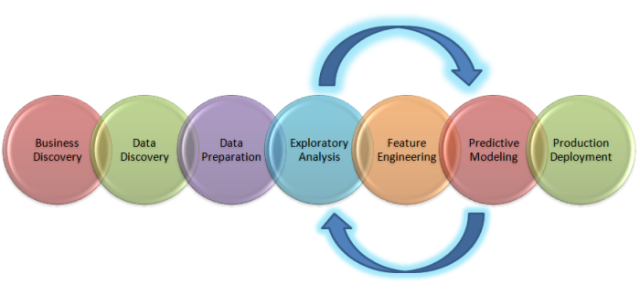
The above figure is a depiction of the big picture on what it entails to solve a business problem from a Data Science perspective. Let us deal with each of the components end to end.

In the Beginning …… : Business Discovery

The start of any data science project is with a business problem. The problem we have at hand is to try to predict the end life of large industrial batteries. When we are encountered with such a business problem, the first thing which should come to our mind is on the key variables which will come into play . For this specific example of batteries some of the key variables which determine the state of health of batteries are conductance, discharge , voltage, current and temperature.

The next questions which we need to ask is on the lead indicators or trends within these variables, which will help in solving the business problem. This is where we also have to take inputs from the domain team. For the case of batteries, it turns out that a key trend which can indicate propensity for failure  is drop in conductance values. The conductance of batteries will drop over time, however the rate at which the conductance values drop will be accelerated before points of failure. This is a vital clue which we will have to be cognizant about when we go for detailed exploratory analysis of the variables.

The other key variable which can come into play is the discharge. When a battery is allowed to discharge the voltage will initially drop to a minimum level and then it will regain the voltage. This is called the “Coup de Fouet” effect. Every manufacturer of batteries will prescribes standards and control charts as to how much, voltage can drop and how the regaining process should be. Any deviation from these standards and control charts would mean anomalous behaviors. This is another set of indicator which will have to look out for when we explore data.

In addition to the above two indicators there are many other factors which one would have to be aware of which will indicate failure. During the business exploration phase we have to identify all such factors which are related to the business problem which we are to solve and formulate hypothesis about them. Once we formulate our hypothesis we have to look out for evidences / trends within the data about these hypothesis. With respect to the two variables which we have discussed above some hypothesis we can formulate are the following.

1. Gradual drop in conductance over time entails normal behaviour and sudden drop would mean anomalous behaviour
2. Deviation from manufactured prescribed “Coup de Fouet” effect would indicate anomalous behaviour

When we go about in exploring data, hypothesis like the above will be point of reference in terms of trends which we will have to look out on the variables involved. The more hypothesis we formulate based on domain expertise the better it would be at the exploratory stage. Now that we have seen what it entails within the business discovery phase, let us encapsulate our discussions on key considerations within the business discovery phase

1. Understand the business problem which we are set out to solve
2. Identify all key variables related to the business problem
3. Identify the lead indicators within these variable which will help in solving the business problem.
4. Formulate hypothesis about the lead indicators

Once we are equipped with sufficient knowledge about the problem from a business and domain perspective now its time to look at the data we have at hand.

And then came data ……. : Data Discovery

In the data discovery phase we have to try to understand some critical aspects about how data is captured and how the variables are represented within the data sets. Some of the key considerations during the data discovery phase are the following

• Do we have data pertaining to all the variables and lead indicators which we defined during the business discovery phase ?
• What is the mechanism of data capture ? Does the data capture mechanism differ according to the variables ?
• What is the frequency of data capture ? Does it vary across the variables ?
• Does the volume of data captured, vary according to the frequency and variables involved ?

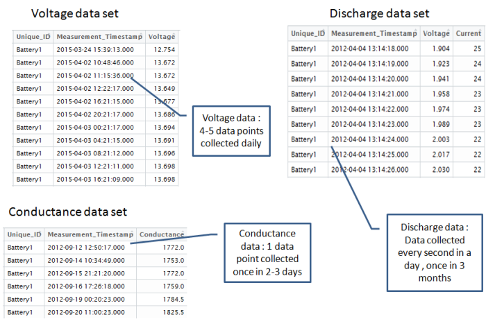
In the case of the battery prediction problem, there are three different data sets . These data sets pertained to different set of variables. The frequency of data collection and the volume of data captured also varies. Some of the key data sets involved are the following

• Conductance data set : Data Pertaining to the conductance of the batteries. This is collected every 2-3 days . Some of the key data points collected along with the conductance data include
  • Time stamp when the conductance data was taken
  • Unique identifier for each battery
  • Other related information like manufacturer , installation location, model , string it was connected to etc
• Terminal voltage data : Data pertaining to Voltage and temperature of battery. This is collected every day. Key data points include
  • Voltage of the battery
  • Temperature
  • Other related information like battery identifier, manufacturer, installation location, model, string data etc
• Discharge Data : Discharge data is collected once every 3 months. Key variable include
  • Discharge voltage
  • Current at which voltage discharges
  • Other related information like battery identifier, manufacturer, installation location, model, string data etc

As seen, we have to play around with three very distinct data sets with different sets of variables, different frequency of time when the data points arrive and different volume of data for each of the variables involved. One of the key challenges, one would encounter is in connecting all these variables together into a coherent data set, which will help in the predictive task. It would be easier to get this done if we can formulate the predictive problem by connecting the data sets available to the business problem we are trying to solve. Let us first attempt to formulate the predictive problem.

Formulating the Predictive Problem : Connecting the dots……

To help formulate the predictive problem, let us revisit the business problem we have at hand and then connect it with the data points which we have at hand.  The predictive problem requires us to predict two things

1. Which battery will fail &
2.  Which period of time in future will the battery fail.

Since the prediction is at a battery level, our unit of reference for formulating the predictive problem is individual battery. This means that all the variables which are present across the multiple data sets have to be consolidated at the individual battery level.

The next question is, at what period of time do we have to consolidate the variables for each battery ? To answer this question, we will have to look at the frequency of data collection for each variable. In the case of our battery data set, the data points for each of the variables are capture at different intervals. In addition the volume of data collected for each of those variables at those instances of time also vary substantially.

• Conductance : One reading of a battery captured once every 3 days.
• Voltage & Temperature : 4-5 readings per battery captured every day.
• Discharge : A set of reading captured every second at different intervals of a day once every 3 months (approximately 4500 – 5000 data points collected in a day).

Since we have to predict the probability of failure at a period of time in future, we will have to have our model learn the behavior of these variables across time periods. However we have to select a time period, where we will have sufficient data points for each of the variables. The ideal time period we should choose in this scenario is every 3 months as discharge data is available only once every 3 months. This would mean that all the data points for each battery for each variable would have to be consolidated to a single record for every 3 months. So if each battery has around 3 years of data it would entail 12 records for a battery.

Another aspect we have to look at is how 3 months of data points for a battery can be consolidated to make one record corresponding to each variable. For this we have to resort to some suitable form of consolidation metric for each variable. What that consolidation metric should be can be finalized after exploratory analysis and feature engineering . We will deal with those aspects in detail when we talk about exploratory analysis and feature engineering phases.

The next important point which we have to deal with would be the labeling of the response variable. Since the business problem is to predict which battery would fail, the response variable would be classifying whether a record of a battery falls under a failure class or not. However there is a lacunae in this approach. What we want is to predict well ahead of time when a battery is likely to fail and therefore we will have to factor in the “when” part also into the classification task. This would entail, looking at samples of batteries which has actually failed and identifying the point of time when failure happened. We label that point as “failure point” and then look back in time from the failure point to classify periods leading to failure. Since the consolidation period for data points is three months, we can fix the “looking back” period also to be 3 months. This would mean, for those samples of batteries where we know the failure point, we look at the record which is one time period( 3 months) before failure and label the data as 1 period before failure, record of data which corresponds to 6 month before failure will be labelled as 2 periods before failure and so on. We can continue labeling the data according to periods before failure, till we reach a comfortable point in time ahead of failure ( say 1 year). If the comfortable period we have in mind is 1 year, we would have 4 failure classes i.e 1 period before failure, 2 periods before failure, 3 periods before failure and 4 periods before failure. All records before the 1 year period of time can be labelled as “Normal Periods”. This labeling strategy will mean that our predictive problem is a multinomial classification problem, with 5 classes ( 4 failure period classes and 1 normal period class).

The above discussed, labeling strategy is for samples of batteries within our data set which have actually failed and where we know when the failure has happened. However if we do not have information about the list of batteries which have failed and which have not failed, we have to resort to intense exploratory analysis to first determine samples of batteries which have failed and then label them according to the labeling strategy discussed above. We can discuss about how we can use exploratory analysis to identify batteries which have failed, in the next post. Needless to say, the records of all batteries which have not failed, will be labelled as “Normal Periods”.

Now that we have seen the predictive problem formulation part, let us recap our discussions so far. The predictive problem formulation step involves the following

1. Understand the business problem and formulate the response variables.
2. Identify the unit of reference to which the business problem will apply ( each battery in our case)
3. Look at the key variables related to the unit of reference and the volume and velocity at which data for these variables are generated
4. Depending on the velocity of data, decide on a data consolidation period and identify the number of records which will be present for the unit of reference.
5. From the data set, identify those units which have failed and which have not failed. Such information will generally be available from past maintenance contracts for each units.
6. Adopt a labeling strategy for both the failed units and normal units. Identify the number of classes which will be applied to all records of the units. For the failed units, label the records as failed classes till a convenient period( 1 year in this case). All records before that period will be labelled the same as the units which have not failed ( “Normal Periods”)

So far we discussed first three phases of the data science process namely business discovery, data discovery and data preparation.The next phase which we will discuss about one of the critical steps of the process namely exploratory. It is in this phase where we leverage the domain knowledge and observe our hypothesis in the data.

Exploratory Analysis – Unravelling latent trends

This phase entails digging deep to get a feel of the data and extract intuitions for feature engineering. When embarking upon exploratory analysis, it would be a good idea to get inputs from domain team on the relation between variables and the business problem. Such inputs are often the starting point for this phase.

Let us now get to the context of our preventive maintenance problem and evolve a philosophy for exploratory analysis.In the case of industrial batteries, a key variable which affects the state of health of a battery is its conductance. It turns out that an indicator of failing health of  battery is the precipitous drop in conductance. Armed with this information our next task should be to  identify, from our available data set,batteries that have higher probability to fail. Since precipitous fall in conductance is an indicator of failing health,the conductance data of  unhealthy batteries will have more variance than the normal ones. So the best way to identify failing batteries from the normal ones would be to apply some consolidating metric like standard deviation or variance on the conductance data and further drill deep on samples which stand apart from the normal population.

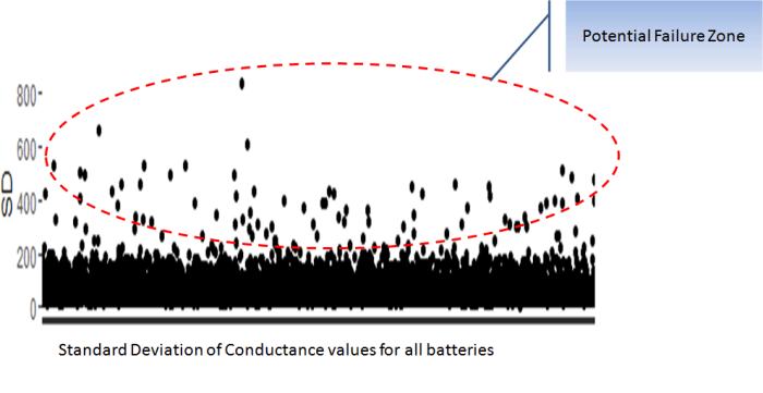
The above is a plot depicting standard deviation of conductance for all batteries. Now what might be of interest to us is the red zone which we can call the “Potential failure Zone”. The potential failure zone consists of those batteries whose conductance values show high standard deviation. Batteries with failing health are likely to exhibit large fall in conductance and as a corollary their values will also show higher standard deviation. This implies that the samples of batteries which have higher probability of failure will in all likelihood be from this failure zone. However to ascertain this hypothesis we will have to dig deep into batteries in the failure zone and look for patterns which might differentiate them from normal batteries. Another objective to dig deep is also to elicit clues from the underlying patterns on what features to include in the predictive model. We will discuss more on the feature extraction when we discuss about feature engineering. Now let us come back to our discussion on digging deep into the failure zone and ferreting out significant patterns. It has to be noted that in addition to the samples in the failure zone we will also have to observe patterns from the normal zone to help separate wheat from the chaff . Intuitions derived by observing different patterns would become vital during feature engineering stage.

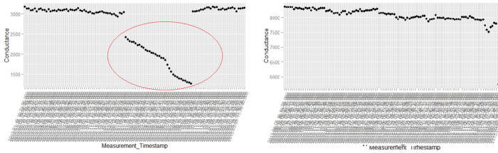
The above figure is a comparison of patterns from either zones. The figure on the left is from the failure zone and the one on the right is from the other. We can clearly see how the precipitous fall is manifested in the sample from the failure zone. The other aspect to note is also the magnitude of the fall. Every battery will have degrading conductance over time. However the magnitude of  degradation is what differentiates the unhealthy  battery from a normal one. We can observe from the plot on the left that the fall in conductance is more than 50%, however for the battery to the right the drop is more muted.  Another aspect we can observe is the slope of conductance. As evident from the two plots, the slope of  conductance profile for the battery on the left is much more steeper over time than the one on the right. These intuitions which we have derived so far might become critical from the overall scheme of feature engineering and modelling. Similar to the intuitions which we have disinterred so far, more could be extracted by observing more samples. The philosophy behind exploratory analysis entails visualizing more and more samples, observing patterns and extracting clues for feature engineering. The more time we spend on doing this more ammunition we get for feature engineering.

Let us now try to encapsulate the philosophy of exploratory analysis in few steps

1. Take inputs from domain team related to the problem we are trying to solve. In our case the clue which we got was the relation between conductance and health of batteries.
2. Identify any consolidating metric for the variable under consideration to separate out anomalous samples. In the example above we used standard deviation of conductance values to find anomalies.
3. Once the samples are demarcated using the consolidation metric, visualize samples from different sets to identify discernible patterns in data.
4. From the patterns we observe root out clues for feature engineering. In our example we identified that % fall in conductance and slope of conductance over time could be potential features.

Multivariate Exploration

So far we were limited to analysis of a single variable i.e conductance. However to get more meaningful insights we have to connect other variables layer by layer to the initial variable which we have analysed to get more insights on the problem. As far as battery is concerned some of the critical variables other than conductance are voltage and discharge. Let us connect these two variables along with the conductance profile to gain more intuitions from the data.

The above figure is a plot which depicts three variables across the same time span. The idea of plotting multiple variables together across a common time span is to unearth any discernible trends we can see together. A cursory look at this plot will reveal some obvious observations.

1. The fall in current and voltage in conjunction with drop in conductance.
2. The cyclic nature of the voltage profile.
3. A gradual drop in the troughs of the voltage profile.

Having made some observations,we now need to ascertain whether these observations can be codified to some definitive trends. This can be verified only by observing plots for many samples of similar variables. By sampling data pertaining to many batteries if we can get similar observations, then we can be sure that we have unearthed some trends explaining behaviors of different variables. However just unearthing some trends will not suffice. We have to get some intuitions from such trends which will help in transforming the raw variables to some form which will help in the modelling task. This is achieved by feature engineering the raw variables.

Feature Engineering

Many a times the given set of raw variables will not suffice for extracting the required predictive power from the model. We will have to transform the raw variables to generate new variables giving us the extra thrust towards better predictive metrics. What transformation has to be done, will be based on the intuitions we build during the exploratory analysis phase and also by combining domain knowledge. For the case of batteries let us revisit some of the intuitions we build during the exploratory analysis phase and see how these intuitions we build can be used for feature engineering.

During our discussions with domain team we found out that precipitous fall in conductance is an indicator of failing health of a battery. So a probable feature we can extract from the conductance variable is the slope of the data points over a fixed time span.The rationale for such a feature is this, if precipitous fall in conductance over time is an indicator of failing health of a battery  then the slope of data points for a battery which is failing will be more steeper than the battery which is healthy. It was observed that through such transformation there was a positive influence on predictive metrics. The dynamics of such transformation is as follows, if we have conductance data for the battery for three years, we can take consecutive three month window of conductance data and take the slope of all the data points and make it as a feature.  By doing this, the number of rows of data for the variable also gets consolidated to much fewer numbers.

Let us also look at another example of feature engineering which we can introduce to the variable, discharge voltage. As seen from the above figure, the discharge voltage follows a wave like profile. It turns out that when a battery discharges the voltage first drops and then it rises. This behavior is called the “Coupe De Fouet” (CDF) effect. Now our thought should be, how do we combine the observed wave like pattern and the knowledge about CDF into a feature ? Again we have to dig into domain knowledge. As per theory on the state of health of batteries there are standards for the CDF profile of a healthy battery and that of a failing battery. These are prescribed by the manufacturer of the battery. For example the manufacturing standards prescribe certain depth to which the voltage will fall during discharge and certain height to which it will go up during a typical CDF effect. The deviance between the observed CDF and the manufacture prescribed standard can be taken as another feature. Similarly we can also think of other features related to voltage, like depth of discharge ( DOD), number of cycles etc. Our focus should be in using the available domain knowledge to transform raw variables into features.

As seen from the above two examples the essence of feature engineering is all about translating the domain knowledge and the trends seen in the data to more meaningful features. The veracity of the models which are built depends a lot on the strength of  the features built. Now that we have seen the feature engineering phase let us now look at modelling strategy for this use case.

Modelling Phase

In the initial part of this article we discussed labelling strategy for training the model. Since the use case is to predict which battery would fail and at what period of time, we have to look back in time from the failure point label for creating different classes related to periods of failure. In this specific case, the different features were created by consolidating 3 months of data into a single row. So one period before failure would denote 3 months before failure. So if the requirement is to predict failure 6 months prior to when it is likely to happen, then we will have 4 different classes i.e  failure point,one period before failure(3 months prior to failure point) ,two periods before failure and (6 months prior to failure point) & normal state. All periods prior to 6 months can be labelled as normal state.

With respect to modelling, we can spot check with different classification algorithms ( logistic regression, Naive bayes, SVM, Random Forest, XGboost .. etc). The choice of final model will be based on the accuracy metrics ( sensitivity , specificity etc) of the spot checked models. Another aspect which might be useful to note is also that, data set could be highly unbalanced i.e the number of normal battery classes is likely to outnumber the failure classes disproportionately. It will be a good idea to try out class balancing methods on the data set before modelling.

Wrapping up

This post brings down curtains to an end to end view of a predictive analytics use case for industrial batteries. Any use case within the manufacturing sector can be quite challenging as the variables involved are very technical and would require lot of interventions from related domain teams. Constant engagement of domain specialist as part of the data science team is very important for the success of such projects.

I have tried my best to write the nuances of such a difficult use case. I have tried to cover the critical elements in the process. In case of any clarifications on the use case and details of its implementation you can connect with me through the following email id bayesianquest@gmail.com. Looking forward to hearing from you.  Till then let me sign off.

Watch this space for more such use cases.