This is the third post of our series on building a self learning recommendation system using reinforcement learning. This series consists of 8 posts where in we progressively build a self learning recommendation system.

1. Recommendation system and reinforcement learning primer
2. Introduction to multi armed bandit problem
3. Self learning recommendation system as a K-armed bandit ( This post )
4. Build the prototype of the self learning recommendation system: Part I
5. Build the prototype of the self learning recommendation system: Part II
6. Productionising the self learning recommendation system: Part I – Customer Segmentation
7. Productionising the self learning recommendation system: Part II – Implementing self learning recommendation
8. Evaluating different deployment options for the self learning recommendation systems.

Introduction

In our previous post we implemented couple of experiments with K-armed bandit. When we discussed the idea of the K-armed bandits from the context of recommendation systems, we briefly touched upon the idea that the buying behavior of a customer depends on the customers context. In this post we will take the idea of the context forward and how the context will be used to build the recommendation system using the K-armed bandit solution.

Defining the context for customer buying

When we discussed about reinforcement learning in our first post, we learned about the elements of a reinforcement learning setting like state, actions, rewards etc. Let us now identify these elements in the context of the recommendation system we are building.

State

When we discussed about reinforcement learning in the first post, we learned that when an agent interacts with the environment at each time step, the agent manifests a certain state. In the example of the robot picking trash the different states were that of high charge or low charge. However in the context of the recommendation system, what would be our states ? Let us try to derive the states from the context of a customer who makes an online purchase. What would be those influencing factors which defines the product the customer buys ? Some of these are

• The segment the customer belongs
• The season or time of year the purchase is made
• The day in which purchase is made

There could be many other influencing factors other than this. For simplicity let us restrict to these factors for now. A state could be made from the combinations of all these factors. Let us arrive at these factors through some exploratory analysis of the data

The data set we would be using is the online retail data set available in the UCI Machine learning library. We will download the data and the place it in local folder and the read the file from the local folder.

import numpy as np
import pandas as pd
from dateutil.parser import parse

Lines 1-3 imports all the necessary packages for our purpose. Let us now load the data as a pandas data frame

# Please use the path to the actual data
filename = "data/Online Retail.xlsx"
# Let us load the customer Details
custDetails = pd.read_excel(filename, engine='openpyxl')
custDetails.head()

In line 5, we load the data from disk and then read the excel shee using the ‘openpyxl’ engine. Please note to pip install the ‘openpyxl’ package if not available.

Let us now parse the date column using date parser and extract information from the date column.

#Parsing  the date
custDetails['Parse_date'] = custDetails["InvoiceDate"].apply(lambda x: parse(str(x)))
# Parsing the weekdaty
custDetails['Weekday'] = custDetails['Parse_date'].apply(lambda x: x.weekday())
# Parsing the Day
custDetails['Day'] = custDetails['Parse_date'].apply(lambda x: x.strftime("%A"))
# Parsing the Month
custDetails['Month'] = custDetails['Parse_date'].apply(lambda x: x.strftime("%B"))
# Getting the year
custDetails['Year'] = custDetails['Parse_date'].apply(lambda x: x.strftime("%Y"))
# Getting year and month together as one feature
custDetails['year_month'] = custDetails['Year'] + "_" +custDetails['Month']
# Feature engineering of the customer details data frame
# Get the date  as a seperate column
custDetails['Date'] = custDetails['Parse_date'].apply(lambda x: x.strftime("%d"))
# Converting date to float for easy comparison
custDetails['Date']  = custDetails['Date'] .astype('float64')
# Get the period of month column
custDetails['monthPeriod'] = custDetails['Date'].apply(lambda x: int(x > 15))

custDetails.head()

As seen from line 11 we have used the lambda() function to first parse the ‘date’ column. The parsed date is stored in a new column called ‘Parse_date’. After parsing the dates first, we carry out different operations, again using the lambda() function on the parsed date. The different operations we carry out are

1. Extract weekday and store it in a new column called ‘Weekday’ : line 13
2. Extract the day of the week and store it in the column ‘Day’ : line 15
3. Extract the month and store in the column ‘Month’ : line 17
4. Extract year and store in the column ‘Year’ : line 19

In line 21 we combine the year and month to form a new column called ‘year_month’. This is done to enable easy filtering of data, based on the combination of a year and month.

We make some more changes from line 24-28. In line 24, we extract the date of the month and then convert it into a float type in line 26. The purpose of taking the date is to find out which of these transactions have happened before 15th of the month and which after 15th. We extract those details in line 28, where we create a binary points ( 0 & 1) as to whether a date falls in the last 15 days or the first 15 days of the month.

We will also create a column which gives you the gross value of each puchase. Gross value can be calculated by multiplying the quantity with unit price. After that we will consolidate the data for each unique invoice number and then explore some of the elements of states which we want to explore

# Creating gross value column
custDetails['grossValue'] = custDetails["Quantity"] * custDetails["UnitPrice"]
# Consolidating accross the invoice number for gross value
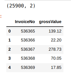
retailConsol = custDetails.groupby('InvoiceNo')['grossValue'].sum().reset_index()
print(retailConsol.shape)
retailConsol.head()

Now that we have got the data consolidated based on each invoice number, let us merge the date related features from the original data frame with this consolidated data. We merge the consolidated data with the custDetails data frame and then drop all the duplicate data so that we get a record per invoice number, along with its date features.

# Merge the other information like date, week, month etc
retail = pd.merge(retailConsol,custDetails[["InvoiceNo",'Parse_date','Weekday','Day','Month','Year','year_month','monthPeriod']],how='left',on='InvoiceNo')
# dropping ALL duplicate values
retail.drop_duplicates(subset ="InvoiceNo",keep = 'first', inplace = True)
print(retail.shape)
retail.head()

Let us first look at the month wise consolidation of data and then plot the data. We will use a functions to map the months to its index position. This is required to plot the data according to months. The function ‘monthMapping‘, maps an integer value to the month and then sort the data frame.

# Create a map for each month
def monthMapping(mnthTrend):
    # Get the map
    mnthMap = {"January": 1, "February": 2,"March": 3, "April": 4,"May": 5, "June": 6,"July": 7, "August": 8,"September": 9, "October": 10,"November": 11, "December": 12}
    # Create a new feature for month
    mnthTrend['mnth'] = mnthTrend.Month
    # Replace with the numerical value
    mnthTrend['mnth'] = mnthTrend['mnth'].map(mnthMap)
    # Sort the data frame according to the month value
    return mnthTrend.sort_values(by = 'mnth').reset_index()

We will use the above function to consolidate the data according to the months and then plot month wise grossvalue data

mnthTrend = retail.groupby(['Month'])['grossValue'].agg('mean').reset_index().sort_values(by = 'grossValue',ascending = False)
# sort the months in the right order
mnthTrend = monthMapping(mnthTrend)
sns.set(rc = {'figure.figsize':(20,8)})
sns.lineplot(data=mnthTrend, x='Month', y='grossValue')
plt.legend(bbox_to_anchor=(1.02, 1), loc='upper left', borderaxespad=0)
plt.show()

We can see that there is sufficient amount of variability of data month on month. So therefore we will take months as one of the context items on which the states can be constructed.

Let us now look at buying pattern within each month and check how the buying pattern is within the first 15 days and the latter half

# Aggregating data for the first 15 days and latter 15 days
fortnighTrend = retail.groupby(['monthPeriod'])['grossValue'].agg('mean').reset_index().sort_values(by = 'grossValue',ascending = False)

sns.set(rc = {'figure.figsize':(20,8)})
sns.lineplot(data=fortnighTrend, x='monthPeriod', y='grossValue')
plt.legend(bbox_to_anchor=(1.02, 1), loc='upper left', borderaxespad=0)
plt.show()

We can see that there is as small difference between buying patterns in the first 15 days of the month and the latter half of the month. Eventhough the difference is not significant, we will still take this difference as another context.

Next let us aggregate data as per the days of the week and and check the trend

# Aggregating data accross weekdays
dayTrend = retail.groupby(['Weekday'])['grossValue'].agg('mean').reset_index().sort_values(by = 'grossValue',ascending = False)

sns.set(rc = {'figure.figsize':(20,8)})
sns.lineplot(data=dayTrend, x='Weekday', y='grossValue')
plt.legend(bbox_to_anchor=(1.02, 1), loc='upper left', borderaxespad=0)
plt.show()

We can also see that there is quite a bit of variability of buying patterns accross the days of the week. We will therefore take the week days also as another context

So far we have observed 4 different features, which will become our context for recommending products. The context which we have defined would act as the states from the reinforcement learning setting perspective. Let us now look at the big picture of how we will formulate the recommendation task as reinforcement learning setting.

The Big Picture

We will now have a look at the big picture of this implementation. The above figure is the representation of what we will implement in code in the next few posts.

The process starts with the customer context, consisting of segment, month, period in the month and day of the week. The combination of all the contexts will form the state. From an implementation perspective we will run simulations to generate the context since we do not have a real system where customers logs in and thereby we automatically capture context.

Based on the context, the system will recommend different products to the customer. From a reinforcement learning context these are the actions which are taken from each state. The initial recommendation of products ( actions taken) will be based on the value function learned from the historical data.

The customer will give rewards/feedback based on the actions taken( products recommended ). The feedback would be the manifestation of the choices the customer make. The choice the customer makes like the products the customer buys, browses and ignores from the recommended list. Depending on the choice made by the customer, a certain reward will be generated. Again from an implementation perspective, since we do not have real customers giving feedback, we will be simulating the customer feedback mechanism.

Finally the update of the value functions based on the reward generated will be done based on the simple averaging method. Based on the value update, the bandit will learn and adapt to the affinities of the customers in the long run.

What next ?

In this post we explored the data and then got a big picture of what we will implement going forward. In the next post we will start implementing these processes and building a prototype using Jupyter notebook. Later on we will build an application using Python scripts and then explore options to deploy the application. Watch out this space for more.

 The next post will be published next week. Please subscribe to this blog post to get notifications when the next post is published.

You can also subscribe to our Youtube channel for all the videos related to this series.

The complete code base for the series is in the Bayesian Quest Git hub repository

Do you want to Climb the Machine Learning Knowledge Pyramid ?

Knowledge acquisition is such a liberating experience. The more you invest in your knowledge enhacement, the more empowered you become. The best way to acquire knowledge is by practical application or learn by doing. If you are inspired by the prospect of being empowerd by practical knowledge in Machine learning, subscribe to our Youtube channel

I would also recommend two books I have co-authored. The first one is specialised in deep learning with practical hands on exercises and interactive video and audio aids for learning

This book is accessible using the following links

The Deep Learning Workshop on Amazon

The Deep Learning Workshop on Packt

The second book equips you with practical machine learning skill sets. The pedagogy is through practical interactive exercises and activities.

This book can be accessed using the following links

The Data Science Workshop on Amazon

The Data Science Workshop on Packt

Enjoy your learning experience and be empowered !!!!