Build you Computer Vision Application – Part III: Pothole detector from scratch using legacy methods (Image Pyramids and sliding window)

This is the third post of the series were we build a road sign and pothole detection application. We will be using multiple methods through out this series which includes computer vision techniques using opencv, annotating images using labelImg, mastering Tensorflow object detection API, Training objection detection using transfer learning, Object detection on video etc. This series will be split across 9 posts.

1. Introduction to object detection

2. Data set preperation and annotation Using labelImg

3. Building your object detection model from scratch using Image pyramids and Sliding window ( This post )

4. Building your road pothole detector using RCNN

5. Building your road pothole detector using YOLO

6. Building you road pothole detector using Tensorflow object detection API

7. Building your video analytics application for detecting potholes

8. Deploying your video analytics application for detection of potholes

In this post we build a custom object detector from scratch progressively using different methods like pyramid segmentation, sliding window and non maxima suppression. These methods are legacy methods which lays the foundation to many of the modern object detection methods. Let us look at the processes which will be covered in building an object detector from scratch.

  1. Prepare the train and test sets from the annotated images ( Covered in the last post)
  2. Build a classifier for detecting potholes
  3. Build the inference pipeline using image pyramids and sliding window techniques to predict bounding boxes for potholes
  4. Optimise the bounding boxes using Non Maxima suppression.

We will be covering all the topics from step 2 in this post. These posts are heavily inspired by the following posts.

Let us dive in.

Training a classifier on the data

In the last post we prepared our training data from positive and negative examples and then saved the data in h5py format. In this post we will use that data to build our pothole classifier. The classifier we will be building is a binary classifier which has a positive class and a negative class. We will be training this classifier using a SVM model. The choice of SVM model is based on some earlier work which is done in this space, however I would urge you to experiment with other classification models as well.

We will start off from where we stopped in the last section. We will read the database from disk and extract the labels and data

# Read the data base from disk
db = h5py.File(outputPath, "r")
# Extract the labels and data
(labels, data) = (db["pothole_features_all"][:, 0], db["pothole_features_all"][:, 1:])
# Close the data base
db.close()

print(labels.shape)
print(data.shape)

We will now use the data and labels to build the classifier

# Build the SVM model
model = SVC(kernel="linear", C=0.01, probability=True, random_state=123)
model.fit(data, labels)

Once the model is fit we will save the model as a pickle file in the output folder.

# Save the model in the output folder
modelPath = 'data/models/model.cpickle'
f = open(modelPath, "wb")
f.write(pickle.dumps(model))
f.close()

Please remember to create the 'models' folder in your local drive in the 'data' folder before saving the model. Once the model is saved you will be able to see the model pickle file within the path you specified.

Now that we have build the classifier, we will use this classifier for object detection in the next section. We will be covering two important concepts in the next section which is important for object detection, Image pyramids and Sliding windows. Let us get familiar with those concepts first.

Image Pyramids and Sliding window techniques

Let us try to understand the concept of image pyramids with an example. Let us assume that we have a window of fixed size and potholes are detected only if they fit perfectly inside the window. Let us look at how well the potholes are detected when using a fixed size window. Take the case of layer1 of the image below. We can see that the fixed sized window was able to detect one of the potholes which was further down the road as it fit well within the window size, however the bigger pothole which is at the near end the image is not detected because the window was obviously smaller than size of the pothole.

As a way to solve this, let us progressively reduce the size of the image, and try to fit the potholes to the fixed window size, as shown in the figure below. With the reduction in size of the image, the object we want to detect also reduces in size. Since our detection window remains the same, we are able to detect more potholes including the biggest one, when the image sizes are reduced. Thereby we will be able to detect most of the potholes which otherwise would not have been possible with a fixed size window and a constant size image. This is the concept behind image pyramids.

The name image pyramids signifies the fact that, if the scaled images are stacked vertically, then it will fit inside a pyramid as shown in the below figure.

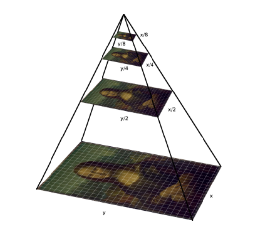
The implementation of image pyramids can be done easily using Sklearn. There are many different types of image pyramid implementation. Some of the prominent ones are Gaussian pyramids and Laplacian pyramids. You can read about these pyramids in the link give here. Let us quickly look at the implementation of of pyramids.

from skimage.transform import pyramid_gaussian
for imgPath in allFiles[-2:-1]:
    # Read the image
    image = cv2.imread(imgPath)
    # loop over the layers of the image pyramid and display them
    for (i, layer) in enumerate(pyramid_gaussian(image, downscale=1.2)):
        # Break the loop if the image size is less than our window size
        if layer.shape[1] < 80 or layer.shape[0] < 40:
            break
        print(layer.shape)

From the output we can see how the images are scaled down progressively.

Having see the image pyramids, its time to discuss about sliding window. Sliding windows are effective methods to identify objects in an image at various scales and locations. As the name suggests, this method involves a window of standard length and width which slides accross an image to extract features. These features will be used in a classifier to identify object of interest. Let us look at the code block below to understand the dynamics of the sliding window method.

# Read the image
image = cv2.imread(allFiles[-2])
# Define the window size
windowSize = [80,40]
# Define the step size
stepSize = 40
# slide a window across the image
for y in range(0, image.shape[0], stepSize):
    for x in range(0, image.shape[1], stepSize):
        # Clone the image
        clone = image.copy()
        # Draw a rectangle on the image 
        cv2.rectangle(clone, (x, y), (x + windowSize[0], y + windowSize[1]), (0, 255, 0), 2)
        plt.imshow()

To implement the sliding window we need to understand some of the parameters which are used. The first is the window size, which is the dimension of the fixed window we would be sliding accross the image. We earlier calculated the size of this window to be [80,40] which was the average size of a pothole in our distribution. The second parameter is the step size. A step size is the number of pixels we need to step to move the fixed window accross the image. Smaller the step size, we will have to move through more pixels and vice-versa. We dont want to slide through every pixel and definitely dont want to skip important features, and therefore the step size is a necessary parameter. An ideal step size would depend on the image size. For our case let us experiment with the ‘y’ cordinate size of our fixed window which is 40. I would encourage to experiment with different step sizes and observe the results before finalising the step size.

To implement this method, we first iterates through the vertical distance starting from 0 to the height of the image with increments of the stepsize. We have an inner iterative loop which loops through the horizontal direction ranging from 0 to the width of the image with increments of stepsize. For each of these iterations we capture the x and y cordinates and then extract a rectangle with the same shape of the fixed window size. In the above implementation we are only drawing a rectangle on the image to understand the dynamics. However when we implement this along with image pyramids, we will crop an image size with the dimension of the window size as we slide accross the image. Let us see some of the sample outputs of the sliding window.

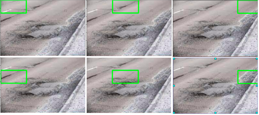
From the above output we can see how the fixed window slides accross the image both horizontally and vertically with a step size to extract features from the image of the same size as the fixed window.

So far we have seen the pyramid and the sliding window implementations independently. These two methods have to be integrated to use it as an object detector. However for integrating them we need to convert the sliding window method into a function. Let us look at the function to implement sliding windows.

# Function to implement sliding window
def slidingWindow(image, stepSize, windowSize):    
    # slide a window across the image
    for y in range(0, image.shape[0], stepSize):
        for x in range(0, image.shape[1], stepSize):
            # yield the current window
            yield (x, y, image[y:y + windowSize[1], x:x + windowSize[0]])

The function is not very different from what we implemented earlier. The only difference is as the output we yield a tuple of the x,y cordinates and the crop of the image of the same size as the window Size. Next we will see how we integrate this function with the image pyramids to implement our custom object detector.

Building the object detector

Its now time to bring all what we defined into creating our object detector. As a first step let us load the model which we saved during the training phase

# Listing the path were we stored the model
modelPath = 'data/models/model.cpickle'
# Loading the model we trained earlier
model = pickle.loads(open(modelPath, "rb").read())
model

Now let us look at the complete code to implement our object detector

# Initialise lists to store the bounding boxes and probabilities
boxes = []
probs = []
# Define the HOG parameters
orientations=12
pixelsPerCell=(4, 4)
cellsPerBlock=(2, 2)
# Define the fixed window size
windowSize=(80,40)
# Pick a random image from the image path to check our prediction
imgPath = sample(allFiles,1)[0]
# Read the image
image = cv2.imread(imgPath)
# Converting the image to grayscale
gray = cv2.cvtColor(image, cv2.COLOR_BGR2GRAY)
# loop over the image pyramid
for (i, layer) in enumerate(pyramid_gaussian(image, downscale=1.2)):
    # Identify the current scale of the image    
    scale = gray.shape[0] / float(layer.shape[0])
    # loop over the sliding window for each layer of the pyramid
    for (x, y, window) in slidingWindow(layer, stepSize=40, windowSize=(80,40)):
        # if the current window does not meet our desired window size, ignore it
        if window.shape[0] != windowSize[1] or window.shape[1] != windowSize[0]:
            continue
        # Let us now extract the hog features of this window within the image
        feat = hogFeatures(window,orientations,pixelsPerCell,cellsPerBlock,normalize=True).reshape(1,-1)
        # Get the prediction probabilities for the positive class ( potholesf)
        prob = model.predict_proba(feat)[0][1] 
        
        # Check if the probability is greater than a threshold probability
        if prob > 0.95:            
            # Extract (x, y)-coordinates of the bounding box using the current scale 
            # Starting coordinates
            (startX, startY) = (int(scale * x), int(scale * y))
            # Ending coordinates
            endX = int(startX + (scale * windowSize[0]))
            endY = int(startY + (scale * windowSize[1]))
            # update the list of bounding boxes and probabilities
            boxes.append((startX, startY, endX, endY))
            probs.append(prob)
            
# loop over the bounding boxes and draw them
for (startX, startY, endX, endY) in boxes:
    cv2.rectangle(image, (startX, startY), (endX, endY), (0, 0, 255), 2)       

plt.imshow(image,aspect='equal')
plt.show() 

To start of we initialise two lists in lines 2-3 where we will store the bounding box coordinates and also the probabilities which indicates the confidence about detecting potholes in the image.

We also define some important parameters which are required for HOG feature extraction method in lines 5-7

  1. orientations
  2. pixels per Cell
  3. Cells per block

We also define the size of our fixed window in line 9

To test our process, we randomly sample an image from the list of images we have and then convert the image into gray scale in lines 11-15.

We then start the iterative loop to implement the image pyramids in line 17. For each iteration the input image is scaled down as per the scaling factor we defined.Next we calculate the running scale of the image in line 19. The scale would always be the original shape divided by the scaled down image. We need to find the scale to blow up the x,y coordinates to the orginal size of the image later on.

Next we start the sliding window implementation in line 21. We provide the scaled down version of the image as the input along with the stepSize and the window size. The step size is the parameter which indicates by how much the window has to slide accross the original image. The window size indicates the size of the sliding window. We saw the mechanics of these when we looked at the sliding window function.

In lines 23-24 we ensure that we only take images, which meets our minimum size specification.For any image which passes the minimum size specification, HOG features are extracted in line 26. On the extracted HOG features, we do a prediction in line 28. The prediction gives the probability whether the image is a pothole or not. We extract only probability of the positive class. We then take only those images were the probability is greater than a threshold we have defined in line 31. We give a high threshold because, our distribution of both the positive and negative images are very similar. So to ensure that we get only the potholes, we given a higher threshold. The threshold has been arrived at after fair bit of experimentation. I would encourage you to try out with different thresholds before finalising the threshold you want.

Once we get the predictions, we take those x and y cordinates and then blow it to the original size using the scale we earlier calculated in lines 34-37. We find the starting cordinates and the ending cordinates and then append those coordinates in the lists we defined, in lines 39-40.

In lines 43-47, we loop through each of the coordinates and draw bounding boxes around the image.

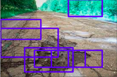
Let us look at the output we have got, we can see that there are multiple bounding boxes created around the area were there are potholes. We can be happy that the object detector is doing its job by localising around the area around a pothole in most of the cases. However there are examples where the detector has detected objects other than potholes. We will come to that issue later. Let us first address another important issue.

All the images have multiple overlapping bounding boxes. Having a lot of bounding boxes can sometimes be cumbersome say if we want to calculate the area where the pot hole is present. We need to find a way to reduce the number of overlapping bounding boxes. This is were we use a technique called Non Maxima suppression. The objective of Non maxima suppression is to combine bounding boxes with significant overalp and get a single bounding box. The method which we would be implementing is inspired from this post

Non Maxima Suppression

We would be implementing a customised method of the non maxima suppression implementation. We will be implementing it through a function.

def maxOverlap(boxes):
    '''
    boxes : This is the cordinates of the boxes which have the object
    returns : A list of boxes which do not have much overlap
    '''
    # Convert the bounding boxes into an array
    boxes = np.array(boxes)
    # Initialise a box to pick the ids of the selected boxes and include the largest box
    selected = []
    # Continue the loop till the number of ids remaining in the box is greater than 1
    while len(boxes) > 1:
        # First calculate the area of the bounding boxes 
        x1 = boxes[:, 0]
        y1 = boxes[:, 1]
        x2 = boxes[:, 2]
        y2 = boxes[:, 3]
        area = (x2 - x1) * (y2 - y1)
        # Sort the bounding boxes based on its area    
        ids = np.argsort(area)
        #print('ids',ids)
        # Take the coordinates of the box with the largest area
        lx1 = boxes[ids[-1], 0]
        ly1 = boxes[ids[-1], 1]
        lx2 = boxes[ids[-1], 2]
        ly2 = boxes[ids[-1], 3]
        # Include the largest box into the selected list
        selected.append(boxes[ids[-1]].tolist())
        # Initialise a list for getting those ids that needs to be removed.
        remove = []
        remove.append(ids[-1])
        # We loop through each of the other boxes and find the overlap of the boxes with the largest box
        for id in ids[:-1]:
            #print('id',id)
            # The maximum of the starting x cordinate is where the overlap along width starts
            ox1 = np.maximum(lx1, boxes[id,0])
            # The maximum of the starting y cordinate is where the overlap along height starts
            oy1 = np.maximum(ly1, boxes[id,1])
            # The minimum of the ending x cordinate is where the overlap along width ends
            ox2 = np.minimum(lx2, boxes[id,2])
            # The minimum of the ending y cordinate is where the overlap along height ends
            oy2 = np.minimum(ly2, boxes[id,3])
            # Find area of the overlapping coordinates
            oa = (ox2 - ox1) * (oy2 - oy1)
            # Find the ratio of overlapping area of the smaller box with respect to its original area
            olRatio = oa/area[id]            
            # If the overlap is greater than threshold include the id in the remove list
            if olRatio > 0.50:
                remove.append(id)                
        # Remove those ids from the original boxes
        boxes = np.delete(boxes, remove,axis = 0)
        # Break the while loop if nothing to remove
        if len(remove) == 0:
            break
    # Append the remaining boxes to the selected
    for i in range(len(boxes)):
        selected.append(boxes[i].tolist())
    return np.array(selected)

The input to the function are the bounding boxes we got after our prediction. Let me give a big picture of what this implementation is all about. In this implementation we start with the box with the largest area and progressively eliminate boxes which have considerable overlap with the largest box. We then take the remaining boxes after elimination and the repeat the process of elimination till we get to the minimum number of boxes. Let us now see this implementation in the code above.

In line 7, we convert the bounding boxes into an numpy array and the initialise a list to store the bounding boxes we want to return in line 9.

Next in line 11, we start the continues loop for elimination of the boxes till the number of boxes which remain is less than 2.

In lines 13-17, we calculate the area of all the bounding boxes and then sort them in ascending order in line 19.

We then take the cordinates of the box with the largest area in lines 22-25 and then append the largest box to the selection list in line 27. We initialise a new list for the boxes which needs to be removed and then include the largest box in the removal list in line 30.

We then start another iterative loop to find the overlap of the other bounding boxes with the largest box in line 32. In lines 35-43, we find the coordinates of the overlapping portion of each of the other boxes with the largest box and the take the area of the overlapping portion. In line 45 we find the ratio of the overlapping area to the original area of the bounding box which we iterate through. If the ratio is larger than a threshold value, we include that box to the removal list in lines 47-48 as this has good overlap with the largest box. After iterating through all the boxes in the list, we will get a list of boxes which has good overlap with the largest box. We then remove all those overlapping boxes and the current largest box from the original list of boxes in line 50. We continue this process till there are no more boxes to be removed. Finally we add the last remaining box to the selected list and then return the selection.

Let us implement this function and observe the result

# Get the selected list
selected = maxOverlap(boxes)

Now let us look at different examples after non maxima suppression.

# Get the image again
image = cv2.imread(imgPath)
# Make a copy of the image
clone = image.copy()
for (startX, startY, endX, endY) in selected:
    cv2.rectangle(clone, (startX, startY), (endX, endY), (0, 255, 0), 2)       

plt.imshow(clone,aspect='equal')
plt.show() 
Non maxima suppression

We can see that the bounding boxes are considerably reduced using our non maxima suppression implementation.

Improvement Opportunities

Eventhough we have got reasonable detection effectiveness, is the model we built perfect ? Absolutely not. Let us look at some of the major pitfalls

Misclassifications of objects :

From the outputs, we can see that we have misclassified some of the objects.

Most of the misclassifications we have seen are for vegetation. There are also cases were road signs are also misclassified as potholes.

A major reason we have mis classification is because our training data is limited. We used only 19 positive images and 20 negative examples. Which is a very small data set for tasks like this. Considering the fact that the data set is limited the classifier has done a decent job. Also for negative images, we need to include some more variety, like get some road signs, vehicles, vegetation etc labelled as negative images. So with more positive images and more negative images with little more variety of objects that are likely to be found on roads will improve the classification accuracy of the classifier.

Another strategy is to experiment with different types of classifiers. In our example we used a SVM classifier. It would be worthwhile to use other binary classifiers starting from Logistic regression, Naive Bayes, Random forest, XG boost etc. I would encourage you to try out with different classifiers and then verify the results.

Non detection of positive classes

Along with misclassifications, we have also seen non detection of positive classes.

As seen from the examples, we can see that there has been non detection in cases of potholes with water in it. In addition some of the potholes which are further along the road are not detected.

These problems again can be corrected by including more variety in the positive images, by including potholes with water in it. It will also help to include images with potholes further away along the road. The other solution is to preprocess images with different techniques like smoothing and blurring, thresholding, gradient and edge detection, contours, histograms etc. These methods will help in highliging the areas with potholes which will help in better detection. In addition, increasing the number of positive examples will also help in addressing the problems associated with non detection.

What Next ?

The idea behind this post was to give you a perspective in building an object detector from scratch. This was also an attempt to give an experience in working in cases where the data sets are limited and where you have to create the necessary data sets. I believe these exercises will equip you will capabilities to deal with such issues in your projects.

Now that you have seen the basic grounds up approach, it is time to use this experience to learn more state of the art techniques. In the next post we will start with more advanced techniques. We will also be using transfer learning techniques extensively from the next post. In the next post we will cover object detection using RCNN.

To be notified of the next post please subscribe to this blog post .You can also subscribe to our Youtube channel for all the videos related to this series.

You can also access the code base for this series from the following git hub link

Do you want to Climb the Machine Learning Knowledge Pyramid ?

Knowledge acquisition is such a liberating experience. The more you invest in your knowledge enhacement, the more empowered you become. The best way to acquire knowledge is by practical application or learn by doing. If you are inspired by the prospect of being empowerd by practical knowledge in Machine learning, subscribe to our Youtube channel

I would also recommend two books I have co-authored. The first one is specialised in deep learning with practical hands on exercises and interactive video and audio aids for learning

This book is accessible using the following links

The Deep Learning Workshop on Amazon

The Deep Learning Workshop on Packt

The second book equips you with practical machine learning skill sets. The pedagogy is through practical interactive exercises and activities.

The Data Science Workshop Book

This book can be accessed using the following links

The Data Science Workshop on Amazon

The Data Science Workshop on Packt

Enjoy your learning experience and be empowered !!!!

Build you Computer Vision Application – Part II: Data preperation and Annotation

This is the second post of the series were we build a road sign and pothole detection application. We will be using multiple methods through out this series which includes computer vision techniques using opencv, annotating images using labelImg, mastering Tensorflow object detection API, Training objection detection using transfer learning, Object detection on video etc. This series will be split across 8 posts.

1. Introduction to object detection

2. Data set preperation and annotation Using labelImg ( This Post )

3. Building your road pothole detector from scratch using Image pyramids and Sliding window

4. Building your road pothole detector using RCNN

5. Building your road pothole detector using YOLO

6. Building you road pothole detector using Tensorflow object detection API

7. Building your video analytics application for detecting potholes

8. Deploying your video analytics application for detection of potholes

In this post we will talk about the data annotation and data preperation stage of the process

Data Sets for Object Detection

In the last post we got introduced to Object detection tasks. We also briefly discovered some of the leading approaches for object detection. When discussing about model training approaches you would have identified that the data sets for object detection are not exactly like any data sets which you would have encountered in your normal machine learning lifecycle. Object detection data sets have two sets of labels, one is the class label for the objects and the second is the bounding boxes for each of the object. The bounding boxes contains the (x ,y )cordinates of the four corners where the object is present. There are different publicly available data sets for object detection tasks. The coco dataset being one of the most popular ones

For the specific task which we are dealing with i.e. Pothole detection, we might not have annotated data sets. Therefore we will have to create that dataset which includes the class labels and the bounding boxes.

This post will talk about downloading data for pothole detection, creating the class labels and bounding boxes for the data and then extracting the necessary information from the annotation task so that we can use it for training the data set. In this exercise we will use a tool called labelIMG which will be used for annotating the dataset.

Installing and Configuraing labelIMG

LabelImg is a free, open source tool for graphically labeling images. It’s written in Python and is an easy, free way to label images for your object detection projects.

Installation of labelImg is quite simple and it can be installed using pip command for python3 as shown below.

pip3 install labelImg

To know more about the installation and configuration you can refer the following link.

Lets now look at how we collect data and annotate them using labelImg

Raw Data Creation

The first task is to create the data set required for training the model and also annotation. The images which are used in this series are collected from google images.

You can download as many images as you want for this task. Always remember to get some good variety of images with different type of objects which you are likely to see on roads.

Annotation of the images

The annotation of the images are done using labelImg application.

To activate the labelImg application, just invoke the labelImg command on the terminal as follows

Figure 1 : Activating labelIMG on terminal

Once this is activated a front end will be opened as follows

Figure 2 : Front end of labelIMg

We start with selecting the directory where the files are stored. We select the directory using the open Dir icon. Once we select the Open Dir icon we will get all the images in the direcotry listed in the application as follows

Figure 3 : Files list

We navigate one image at a time, and then draw the bounding boxes of the objects we want to annotate. Once the bounding boxes are drawn we can input the label we want to give to the image. Once the bounding boxes are selected and annotation are done, the image can be saved as an xml file.

Figure 4 : Annotating the images

Let us open one fo the xml files and look at the information contained in the xml file. The xml file contains the bounding boxes and the class information of the images as shown below.

Figure 5 : xml file information

We have now annotated all the files with the class names and bounding boxes. Let us now extract the information from the xml files into a csv files

Extracting the Information from annotation

In this section we will extract all the annotation information into a pandas data frame and later on to csv file. We will start with importing all the library files we require.

import os
import glob
import pandas as pd
import xml.etree.ElementTree as ET

Next let us list down all the ‘xml’files in the folder using glob() method. We have to give the path of the folder where all the xml files are stored.

# Define the path
path = 'data'
# Get the list of all files in the folder
allFiles = glob.glob(path + '/*.xml')
allFiles
Figure 6 : List of all xml files

Next we need to parse through the 'xml'files and then extract the information from the file. We will use the 'ElementTree' method in the xml package to parse through the folder and then get the relevant information.

# Get one of the files
xml_file = allFiles[0]
# Parse xml file and get the root
tree = ET.parse(xml_file)
root = tree.getroot()
# For each element of the root print the tag and the attribute
for child in root:
    print(child.tag, child.attrib)
Figure 7 : Extracted elements from xml file

In line 13 -14 we get the 'tree' object and the get the 'root' of the xml file. The root contains all the elements as children. Lines 16-17 we go through each of the elements of the xml file and then extract the tags and the attribute of the element. We can see the major elements printed. If we look at the raw xml file we can see all these elements listed there.

As seen in the output, elements named as ‘object’ are the bounding boxes we annotated in the earlier step. These objects contains the bounding box information we need. Before we extract the bounding box information, let us look at some basic methods to extract any information from the root.

filename = root.find('filename').text
filename
Output : Name of the xml file

In line 18 we extract the filename of this xml file using the root.find() method. We need to specify which element we want to look into, which in our case is the text called ‘filename‘ as that is how it is represented in the xml file. To get the filename as a string we give the .text extension.

Let us now get the width and height of the image. We can see from the xml file that this is contained in the element, 'size'

# Extract width and height of the image
width = int(root.find('size').find('width').text)
height = int(root.find('size').find('height').text)
print(width,height)

In lines 21-22 use the find() method to extract width and height and then convert the text into integer.

Our next task is to extract the class names and the bounding box elements. These are contained in each of the 'object' elements under the name 'bndbox'. The class label of the image is contained inside this element under the element name 'name' and the bounding boxes are with the element names 'xmin','ymin','xmax','ymax'. Let us look at one of the sample object elements.

# Get all the 'object' elements
members = root.findall('object')
# Take the first one to extract the information as an example
member = members[0]
print(member.find('name').text)
print(member.find('bndbox').find('xmin').text)
Class label and x min coordinate of the object

From lines 28-29 we can see the class name and one of the bounding box values extracted using the find() method as seen before

Now that we have seen all the moving parts , let us encapsulate all these into a function and extract all the information into a pandas dataframe. This code is taken from this tutorial link for object detection.

def xml_to_pd(path):
    """Iterates through all .xml files (generated by labelImg) in a given directory and combines
    them in a single Pandas dataframe.

    Parameters:
    ----------
    path : str
        The path containing the .xml files
    Returns
    -------
    Pandas DataFrame
        The produced dataframe
    """

    xml_list = []
    # List down all the files within the path
    for xml_file in glob.glob(path + '/*.xml'):
        # Get the tree and the root of the xml files
        tree = ET.parse(xml_file)
        root = tree.getroot()
        # Get the filename, width and height from the respective elements
        filename = root.find('filename').text
        width = int(root.find('size').find('width').text)
        height = int(root.find('size').find('height').text)
        # Extract the class names and the bounding boxes of the classes
        for member in root.findall('object'):
            bndbox = member.find('bndbox')
            value = (filename,
                     width,
                     height,
                     member.find('name').text,
                     int(bndbox.find('xmin').text),
                     int(bndbox.find('ymin').text),
                     int(bndbox.find('xmax').text),
                     int(bndbox.find('ymax').text),
                     )
            xml_list.append(value)
    # Consolidate all the information into a data frame
    column_name = ['filename', 'width', 'height',
                   'class', 'xmin', 'ymin', 'xmax', 'ymax']
    xml_df = pd.DataFrame(xml_list, columns=column_name)
    return xml_df

Let us now extract the information of all the xml files and then convert it into a pandas data frame.

pothole_df = xml_to_pd(path)
pothole_df
Pandas dataframe containing the bounding box information

Finally let us save this label information in a csv file as we will use it later for training our object detection elements.

pothole_df.to_csv('pothole_df.csv',index=False)

Having prepared the data set, let us now look at the next process which is to prepare the train and test sets.

Preparing the Training and test sets

The process of building the train images, involves multiple processes. Let us look at each of them

Mixing positive and negative images

We just annotated the images with potholes along with its bounding boxes. We will be using those images for building the positive classes for the object detector. Along with the positive classes, we also need to get some negative examples. For negative examples we will take some examples of roads without potholes. We will keep both the positive and negative examples, in seperate folders and then use them for building the training data. We will also use some augmentation techniques to increase the training data. Let us dive deeper with the preperation of the training data set.

import os
import glob
import pandas as pd
import io
import cv2
from skimage import feature
import skimage
from sklearn.feature_extraction.image import extract_patches_2d
from sklearn.svm import SVC
import numpy as np
import argparse
import pickle
import matplotlib.pyplot as plt
from random import sample
%matplotlib inline

We will start by importing all the required packages. Next let us look at the positive examples, which are the images with potholes that were downloaded in the last post.

# Positive Images
path = 'data'
allFiles = glob.glob(path + '/*.jpeg')
print(len(allFiles))
allFiles

The above figure lists the images which were downloaded and annotated earlier. You are free to download any number of images. The more the better, as the classifier will perform well with more examples. Later on we will see how we augment these images with different augmentation techniques to increase the number of positive images. However whatever the type of augmentation techniques we use, it would still not be a substitute for variety of positive images.

Let us now look at the negative classes of images. For negative classes we will be using images of normal roads. Let us look at some of the examples of the negative images

# Negative images
path = 'data/Annotated'
roadFiles = glob.glob(path + '/*.jpeg')
for imgPath in roadFiles[:2]:
    img = cv2.imread(imgPath)
    plt.imshow(img)
    plt.show()

These negative images were downloaded in the same way the positive images were also downloaded i.e. from Google images. Again more the examples the better. However what needs to be noted is to maintain a fair balance between the positive and negative examples.

Extracting HOG features from the images

Once the positive and negative images are collected, its now the turn to extract features from the images. There a different methods to extract features from images. The method we will be using is the HOG features. HOG stands for ‘Histogram of Oriented Gradients’. Let us quickly take a quick tour of the HOG method.

Histogram of Oriented Gradients ( HOG )

HOG descriptors are used to represent the structure and appearence of the object in an image. This algorithm works on the principle that an object in an image can be modeled by the distribution of intensity gradients within regions where the object reside. The implementation of this method entails dividing an image into small cells and then for each cell computing the histogram of oriented gradients for pixels within each cell. The histograms accross multiple cells are accumulated to form the feature vector. The dimensionality of these feature vectors depend on the dimension of the image and the parameters of the HOG descriptor like pixels_per_cell, cells_per_block and orientations. You can refer to the following link to learn more about HOG descriptors

Let us now implement the methods for extracting the features and saving the data set on to disk. As a first step we will read the positive images which are the pothole images. We will read the data from the information in the csv file we created earlier. We will take the information and then extract only those patches which contain potholes. Let us first look at the csv file containing the data.

# Reading the csv file
pothole_df = pd.read_csv('pothole_df.csv')
pothole_df

As seen from the output, the data set extracted here contains only 65 rows which comprises of all the classes including vegetation, signs, potholes etc. From this csv file, we will extract only the pothole data. The number of images have been kept intentionally low, so that we can also explore some augmentation techniques so as to enhance the data set. When you embark on custom solutions where data sets are not available you will have to resort to different augmentation techniques to improve your results.

Let us now exlore the dimensions of the set of potholes images we have, and then look at the average width and height of the bounding boxes. This, as we will see later, is to define the width of the window for the pyramid and sliding window techniques. We will use pothole_df data frame to find the dimensions.

# Find the mean of the x dim and y dimensions of the pothole class
xdim = np.mean(pothole_df[pothole_df['class']=='pothole']['xmax'] - pothole_df[pothole_df['class']=='pothole']['xmin'])
ydim = np.mean(pothole_df[pothole_df['class']=='pothole']['ymax'] - pothole_df[pothole_df['class']=='pothole']['ymin'])
print(xdim,ydim)

We will round off the dimensions to [80,40] which we will adopt as the window dimensions for the pyramid and sliding window methods.

# We will take the windows dimension as these dimensions rounded off
winDim = [80,40]

Once the images are read from the excel sheet, its time to extract the patches of potholes which we require, from the images. There are two functions which we require to extract the features which we want. The first one is to extract the hog features from the image. Let us look at that function first.

# Defining the hog structure
def hogFeatures(image,orientations,pixelsPerCell,cellsPerBlock,normalize=True):
    # Extracting the hog features from the image
    feat = feature.hog(image, orientations=orientations, pixels_per_cell=pixelsPerCell,cells_per_block = cellsPerBlock, transform_sqrt = normalize, block_norm="L1")
    feat[feat < 0] = 0
    return feat

The inputs to this function are the images from which we want to extract the features, the orientations, pixels per cell, cells per block and the normalize flag.

In line 40, we extract the features using feature.hog() method from the image. We provide all our parameters to the method to get the features. Once we extract the features, we remove all the negative pixels by making them as 0 in line 41. The extracted features are then returned by the function in the last line.

The next method we will see is the one to augment our images. There are different types of augmentation techniques which are useful. We will be using techniques like flipping ( both horizontal and vertical flipping) and then rotating them to diffrent angles. Let us see the function to augment our images.

# Defining the function for image augmentation
def imgAug(roi,ht,wd,extensive=True):
    # Initialise the empty list to store images
    rois = []
    # resize the ROI to the desired size
    roi = cv2.resize(roi, (ht,wd), interpolation=cv2.INTER_AREA)
    # Append the different images
    rois.append(roi)
    # Augment the image by flipping both horizontally and vertically
    rois.append(cv2.flip(roi, 1))
    if extensive:        
        rois.append(cv2.flip(roi, 0))
        rois.append(cv2.rotate(roi, cv2.ROTATE_90_CLOCKWISE))
        rois.append(cv2.rotate(roi, cv2.ROTATE_90_COUNTERCLOCKWISE))
        # Rotate to other angles
        for rot in [15,45,60,75,85]:
            # Get the rotation matrix
            rotMatrix = cv2.getRotationMatrix2D((ht/2,wd/2),rot,1)
            # ROtate the matrix using the rotation matrix
            rois.append(cv2.warpAffine(roi,rotMatrix,(ht,wd)))         
    return rois

The inputs to the function are the patch of image we want to augment along with the dimensions we want to resize the image. We also define a parameter called extensive to check if we want to do all the methods or just a simple horizontal flipping.

We first initialise a list to store all the augmented images in line 46 and then we go ahead and resize the image in line 48. The resized image is then appended to the list in line 50.

The first augmentation technique is implemented in the line 52 where in we flip it horizontally. The parameter 1 stands for flipping along the y axis.

Now if we want to go for extensive augmentation, we proceed with other types of augmentation. The first of these methods are the vertical flip, clockwise rotation and anticlockwise rotations as shown in lines 54-56.

Then we do 5 different rotations based on the list of angles we have specified in line 58. You can try out with more angles of your choice. To do the rotation we first have to define a rotation matrix which is centred along the centre of the image as shown in line 60. We also provide the centre of the image the angle by which we have to rotate and the scaling function as input parameters . We have chosen a scale of 1. You can try different scaling parameters and then see its effect on the image.

Once the rotation matrix is defined, the image is rotated using the method cv2.warpAffine() in line 62. Here we give the patch of image, the rotation matrix and the dimensions of the image as inputs.

We finally append all the augmented images into the list and then return the rois.

The overall process to extract the features consists of two functions as given below.

# Functions to extract the bounding boxes and the hog features
def roiExtractor(row,path):
    img = cv2.imread(path + row['filename'])    
    # Get the bounding box elements
    bb = [int(row['xmin']),int(row['ymin']),int(row['xmax']),int(row['ymax'])]
    # Crop the image
    roi = img[bb[1]:bb[3], bb[0]:bb[2]]
    # Get the list of augmented images
    rois = imgAug(roi,80,40)
    return rois

def featExtractor(rois,data,labels,positive=True):
    for roi in rois:
        # Extract hog features
        feat = hogFeatures(roi,orientations,pixelsPerCell,cellsPerBlock,normalize=True)
        # Append data and labels
        data.append(feat)
        labels.append(int(1))        
    return data,labels

The first of these functions is to read an image based on the information from the csv file and then crop the image based on the bounding box coordinates as shown in lines 66-70. Finally in line 72, we do the augmetation of the cropped image.

The second function takes the augmented images derived using the first function and extract the HOG features from each of them. We append the features in the list data and the labels are appended to 1 as these are the positive examples.

Having seen all the functions let us now see the process of preparing the data sets.

# Extracting pothole patches from the data
path = 'data/'
# Parameters for extracting HOG features
orientations=12
pixelsPerCell=(4, 4)
cellsPerBlock=(2, 2)
# Empty lists to store data and labels
data = []
labels = []
# Looping through the excel sheet rows
for idx, row in pothole_df.iterrows():
    if row['class'] == 'pothole':
        rois = roiExtractor(row,path)
        data,labels = featExtractor(rois,data,labels)

The process is quite straighforward. In lines 86-88, we define the parameters for HOG feature extraction. Then we initialise two empty lists in lines 90-91 to store data and the labels. We then loop through each of the rows of the pothole data frame and the extract the rois and features if the class of the row is ‘pothole’.

That was the positive examples we saw. Its now the turn of extracting features for the negative examples. Let us first list all the negative examples

# Listing all the negative examples
path = 'data/Annotated'
roadFiles = glob.glob(path + '/*.jpeg')
roadFiles
# Looping through the files
for row in roadFiles:
    # Read the image
    img = cv2.imread(row)
    # Extract patches
    patches = extract_patches_2d(img,(80,40),max_patches=10)
    # For each patch do the augmentation
    for patch in patches:        
        # Get the list of augmented images
        rois = imgAug(patch,80,40,False)
        # Extract the features using HOG        
        for roi in rois:
            feat = hogFeatures(roi,orientations,pixelsPerCell,cellsPerBlock,normalize=True)
            data.append(feat)
            labels.append(int(-1))

In the process for extracting negative examples , we first iterate through the files and then read each file. Since we dont have to crop a specific area within the image, we will adopt a different strategy to augment images. We extract certain patches of a fixed window size from the image. This is implemented through a method extract_patches_2d() in Sklearn. The dimension of the window size is based on the dimensions we fixed earlier. We also specify the number of patches we want to extract in line 106. For each of the patch we extract, we do only horizontal flip as it wouldnt make sense to do any other augmentation steps for the images of roads. We then extract the HOG features in line 113 like what we did for the positive examples. The labels for these examples are -1 as this is the negative image.

Having extracted features and the labels, we will now write the data to disk using h5py format.

import h5py
import numpy as np
# Define the output path
outputPath = 'data/pothole_features_all.hdf5'
# Create the database and write method
db = h5py.File(outputPath, "w")
dataset = db.create_dataset('pothole_features_all', (len(data), len(data[0]) + 1), dtype="float")
dataset[0:len(data)] = np.c_[labels, data]
db.close()

In this implementation we first define the outputPath and then create the database using the ‘write’ method. To create the dataset we use the create_dataset() method giving the name and the dimensions of the dataset. We increase the second dimenstion with +1 as we will be storing the label also in the same dataset. We finally store the dataset as numpy array where the labels and data are concatenated using the np.c_ method of numpy. After this step the new data base will get created in the specified path.

We can read the database using the h5py.File() method. Let us look at the name of the data set we earlier gave by taking the keys() of the database

# Read the h5py file
db = h5py.File(outputPath)
list(db.keys())
# Shape of the data
db["pothole_features_all"].shape

You can see that the shape of the data set we created. We had 730 examples of both the positive and negative examples . We can also see that we have 8209 features, which is a combination of label + the hog features of 8208.

That takes us to the end of the data preperation stage for building our object detector. In the next post we will take this data and build our object detector from scratch.

What Next ?

In the next post, we will explore different techniques to build our custom object detector. We will be covering the following topics in the next post

  1. Building a classifier using the training data
  2. Introduce the concept of Image pyramids and sliding windows
  3. Using Image pyramids and sliding windows to extract bouding boxes for your images
  4. Use non maxima suppression to eliminate overlap of bounding boxes.

We will be covering lot of ground in the next post. The next post will be published next week. To be notified of the next post please subscribe to this blog post .You can also subscribe to our Youtube channel for all the videos related to this series.

You can also access the code base for this series from the following git hub link

Do you want to Climb the Machine Learning Knowledge Pyramid ?

Knowledge acquisition is such a liberating experience. The more you invest in your knowledge enhacement, the more empowered you become. The best way to acquire knowledge is by practical application or learn by doing. If you are inspired by the prospect of being empowerd by practical knowledge in Machine learning, subscribe to our Youtube channel

I would also recommend two books I have co-authored. The first one is specialised in deep learning with practical hands on exercises and interactive video and audio aids for learning

This book is accessible using the following links

The Deep Learning Workshop on Amazon

The Deep Learning Workshop on Packt

The second book equips you with practical machine learning skill sets. The pedagogy is through practical interactive exercises and activities.

The Data Science Workshop Book

This book can be accessed using the following links

The Data Science Workshop on Amazon

The Data Science Workshop on Packt

Enjoy your learning experience and be empowered !!!!