This is the sixth post of our series on building a self learning recommendation system using reinforcement learning. This series consists of 8 posts where in we progressively build a self learning recommendation system. This series consists of the following posts
Productionising the self learning recommendation system: Part I – Customer Segmentation ( This post )
Productionising the self learning recommendation system: Part II – Implementing self learning recommendation
Evaluating different deployment options for the self learning recommendation systems.
This post builds on the previous post where we started off with building the prototype of the application in Jupyter notebooks. In this post we will see how to convert our prototype into Python scripts. Converting into python script is important because that is the basis for building an application and then deploying them for general consumption.
File Structure for the project
First let us look at the file structure of our project.
The directory RL_Recomendations is the main directory which contains other folders which are required for the project. Out of the directories rlreco is a virtual environment we will create and all our working directories are within this virtual environment.Along with the folders we also have the script rlRecoMain.py which is the main driver script for the application. We will now go through some of the steps in creating this folder structure
When building an application it is always a good practice to create a virtual environment and then complete the application build process within the virtual environment. We talked about this in one of our earlier series for building machine translation applications . This way we can ensure that only application specific libraries and packages are present when we deploy our application.
Let us first create a separate folder in our drive and then create a virtual environment within that folder. In a Linux based system, a seperate folder can be created as follows
$ mkdir RL_Recomendations
Once the new directory is created let us change directory into the RL_Recomendations directory and then create a virtual environment. A virtual environment can be created on Linux with Python3 with the below script
RL_Recomendations $ python3 -m venv rlreco
Here the rlreco is the name of our virtual environment. The virtual environment which we created can be activated as below
RL_Recomendations $ source rlreco/bin/activate
Once the virtual environment is enabled we will get the following prompt.
(rlreco) ~$
In addition you will notice that a new folder created with the same name as the virtual environment. We will use that folder to create all our folders and main files required for our application. Let us traverse through our driver file and then create all the folders and files required for our application.
Create the driver file
Open a file using your favourite editor and name it rlRecoMain.py and the insert the following code.
import argparse
import pandas as pd
from utils import Conf,helperFunctions
from Data import DataProcessor
from processes import rfmMaker,rlLearn,rlRecomend
from utils import helperFunctions
import os.path
from pymongo import MongoClient
Lines 1-2 we import the libraries which we require for our application. In line 3 we have to import Conf class from the utils folder.
So first let us create a folder called utils, which will have the following file structure.
The utils folder has a file called Conf.py which contains the Conf class and another file called helperFunctions.py . The first file controls the configuration functions and the second file contains some of the helper functions like saving data into pickle files. We will get to that in a moment.
First let us open a new python file Conf.py and copy the following code.
from json_minify import json_minify
import json

class Conf:

    def __init__(self,confPath):
        # Read the json file and load it into a dictionary
        conf = json.loads(json_minify(open(confPath).read()))
        self.__dict__.update(conf)
    def __getitem__(self, k):
        return self.__dict__.get(k,None)
The Conf class is a simple class, with its constructor loading the configuration file which is in json format in line 8. Once the configuration file is loaded the elements are extracted by invoking ‘conf’ method. We will see more of how this is used later.
We have talked about the Conf class which loads the configuration file, however we havent made the configuration file yet. As you may know a configuration file contains all the parameters in the application. Let us see the directory structure of the configuration file.
Figure : config folder and configuration file
You can now create the folder called config, under the rlreco folder and then open a file in your editor and then name it custprof.json and include the following code.
As you can see the config, file contains all the configuration items required as part of the application. The first part is where the paths to the raw file and processed pickle files are stored. The second part is the mapping of the column names in the raw file and the names used in our application. The third part contains all the parameters required for the application. The Conf class which we earlier saw will read the json file and all these parameters will be loaded to memory for us to be used in the application.
Lets come back to the utils folder and create the second file which we will name as helperFunctions.py and insert the following code.
from pickle import load
from pickle import dump
import numpy as np


# Function to Save data to pickle form
def save_clean_data(data,filename):
    dump(data,open(filename,'wb'))
    print('Saved: %s' % filename)

# Function to load pickle data from disk
def load_files(filename):
    return load(open(filename,'rb'))
This file contains two functions. The first function starting in line 7 saves a file in pickle format to the specified path. The second function in line 12, loads a pickle file and return the data. These two functions are handy functions which will be used later in our project.
We will come back to the main file rlRecoMain.py and look at the next folder and methods on line 4. In this line we import DataProcessor method from the folder Data . Let us take a look at the folder called Data.
Create the data processor module
The class and the methods associated with the class are in the file dataLoader.py. Let us first create the folder, Data and then open a file named dataLoader.py and insert the following code.
import os
import pandas as pd
import pickle
import numpy as np
import random
from utils import helperFunctions
from datetime import datetime, timedelta,date
from dateutil.parser import parse

class DataProcessor:
    def __init__(self,configfile):
        # This is the first method in the DataProcessor class
        self.config = configfile

     # This is the method to load data from the input files
    def dataLoader(self):
        inputPath = self.config["inputData"]
        dataFrame = pd.read_csv(inputPath,encoding = "ISO-8859-1")
        return dataFrame

    # This is the method for parsing dates
    def dateParser(self):
        custDetails = self.dataLoader()
        #Parsing  the date
        custDetails['Parse_date'] = custDetails[self.config["order_date"]].apply(lambda x: parse(x))
        # Parsing the weekdaty
        custDetails['Weekday'] = custDetails['Parse_date'].apply(lambda x: x.weekday())
        # Parsing the Day
        custDetails['Day'] = custDetails['Parse_date'].apply(lambda x: x.strftime("%A"))
        # Parsing the Month
        custDetails['Month'] = custDetails['Parse_date'].apply(lambda x: x.strftime("%B"))
        # Getting the year
        custDetails['Year'] = custDetails['Parse_date'].apply(lambda x: x.strftime("%Y"))
        # Getting year and month together as one feature
        custDetails['year_month'] = custDetails['Year'] + "_" +custDetails['Month']

        return custDetails

    def gvCreator(self):
        custDetails = self.dateParser()
        # Creating gross value column
        custDetails['grossValue'] = custDetails[self.config["prod_qnty"]] * custDetails[self.config["unit_price"]]

        return custDetails
The constructor of the DataProcessor class takes the config file as the input and then make it available for all the other methods in line 13.
This dataProcessor class will have three methods, dataLoader, dateParser and gvCreator. The last method is the driving method which internally calls other two methods. Let us look at the gvCreator method.
The dateParser method is called first within the gvCreator method in line 40. The dateParser method in turn calls the dataLoader method in line 23. The dataLoader method loads the customer data as a pandas data frame in line 18 and the passes it to the dateParser method in line 23. The dateParser method takes the custDetails data frame and then extracts all the date related fields from lines 25-35. We saw this in detail during the prototyping phase in the previous post.
Once the dates are parsed in the custDetails data frame, it is passed to gvCreator method in line 40 and then the ‘gross value’ is calcuated by multiplying the unit price and the product quantity. Finally the processed custDetails file is returned.
Now we will come back to the rlRecoMain file and the look at the three other classes, rfmMaker,rlLearn,rlRecomend, we import in line 5 of the file rlRecoMain.py. This is imported from the ‘processes’ folder. Let us look at the composition of the processes folder.
We have three files in the folder, processes.
The first one is the __init__.py file which is the constructor to the package. Let us see its contentes. Open a file and name it __init__.py and add the following lines of code.
from .rfmProcess import rfmMaker
from .selfLearnProcess import rlLearn,rlRecomend
Create customer segmentation modules
In lines 1-2 of the constructor file we make the three classes ( rfmMaker,rlLearn and rlRecomend) available to the package. The class rfmMaker is in the file rfmProcess.py and the other two classes are in the file selfLearnProcess.py.
Let us open a new file, name it rfmProcess.py and then insert the following code.
import sys
sys.path.append('path_to_the_folder/RL_Recomendations/rlreco')
import pandas as pd
import lifetimes
from sklearn.cluster import KMeans
from utils import helperFunctions


class rfmMaker:
    def __init__(self,custDetails,conf):
        self.custDetails = custDetails
        self.conf = conf

    def rfmMatrix(self):
        # Converting data to RFM format
        RfmAgeTrain = lifetimes.utils.summary_data_from_transaction_data(self.custDetails, self.conf['customer_id'], 'Parse_date','grossValue')
        # Reset the index
        RfmAgeTrain = RfmAgeTrain.reset_index()
        return RfmAgeTrain

    # Function for ordering cluster numbers

    def order_cluster(self,cluster_field_name, target_field_name, data, ascending):
        # Group the data on the clusters and summarise the target field(recency/frequency/monetary) based on the mean value
        data_new = data.groupby(cluster_field_name)[target_field_name].mean().reset_index()
        # Sort the data based on the values of the target field
        data_new = data_new.sort_values(by=target_field_name, ascending=ascending).reset_index(drop=True)
        # Create a new column called index for storing the sorted index values
        data_new['index'] = data_new.index
        # Merge the summarised data onto the original data set so that the index is mapped to the cluster
        data_final = pd.merge(data, data_new[[cluster_field_name, 'index']], on=cluster_field_name)
        # From the final data drop the cluster name as the index is the new cluster
        data_final = data_final.drop([cluster_field_name], axis=1)
        # Rename the index column to cluster name
        data_final = data_final.rename(columns={'index': cluster_field_name})
        return data_final

    # Function to do the cluster ordering for each cluster
    #

    def clusterSorter(self,target_field_name,RfmAgeTrain, ascending):
        # Defining the number of clusters
        nclust = self.conf['nclust']
        # Make the subset data frame using the required feature
        user_variable = RfmAgeTrain[['CustomerID', target_field_name]]
        # let us take four clusters indicating 4 quadrants
        kmeans = KMeans(n_clusters=nclust)
        kmeans.fit(user_variable[[target_field_name]])
        # Create the cluster field name from the target field name
        cluster_field_name = target_field_name + 'Cluster'
        # Create the clusters
        user_variable[cluster_field_name] = kmeans.predict(user_variable[[target_field_name]])
        # Sort and reset index
        user_variable.sort_values(by=target_field_name, ascending=ascending).reset_index(drop=True)
        # Sort the data frame according to cluster values
        user_variable = self.order_cluster(cluster_field_name, target_field_name, user_variable, ascending)
        return user_variable


    def clusterCreator(self):

        #data : THis is the dataframe for which we want to create the clsuters
        #clustName : This is the variable name
        #nclust ; Numvber of clusters to be created

        # Get the RFM data Frame
        RfmAgeTrain = self.rfmMatrix()
        # Implementing for user recency
        user_recency = self.clusterSorter('recency', RfmAgeTrain,False)
        #print('recency grouping',user_recency.groupby('recencyCluster')['recency'].mean().reset_index())
        # Implementing for user frequency
        user_freqency = self.clusterSorter('frequency', RfmAgeTrain, True)
        #print('frequency grouping',user_freqency.groupby('frequencyCluster')['frequency'].mean().reset_index())
        # Implementing for monetary values
        user_monetary = self.clusterSorter('monetary_value', RfmAgeTrain, True)
        #print('monetary grouping',user_monetary.groupby('monetary_valueCluster')['monetary_value'].mean().reset_index())

        # Merging the individual data frames with the main data frame
        RfmAgeTrain = pd.merge(RfmAgeTrain, user_monetary[["CustomerID", 'monetary_valueCluster']], on='CustomerID')
        RfmAgeTrain = pd.merge(RfmAgeTrain, user_freqency[["CustomerID", 'frequencyCluster']], on='CustomerID')
        RfmAgeTrain = pd.merge(RfmAgeTrain, user_recency[["CustomerID", 'recencyCluster']], on='CustomerID')
        # Calculate the overall score
        RfmAgeTrain['OverallScore'] = RfmAgeTrain['recencyCluster'] + RfmAgeTrain['frequencyCluster'] + RfmAgeTrain['monetary_valueCluster']
        return RfmAgeTrain

    def segmenter(self):

        #This is the script to create segments after the RFM analysis

        # Get the RFM data Frame
        RfmAgeTrain = self.clusterCreator()
        # Segment data
        RfmAgeTrain['Segment'] = 'Q1'
        RfmAgeTrain.loc[(RfmAgeTrain.OverallScore == 0), 'Segment'] = 'Q2'
        RfmAgeTrain.loc[(RfmAgeTrain.OverallScore == 1), 'Segment'] = 'Q2'
        RfmAgeTrain.loc[(RfmAgeTrain.OverallScore == 2), 'Segment'] = 'Q3'
        RfmAgeTrain.loc[(RfmAgeTrain.OverallScore == 4), 'Segment'] = 'Q4'
        RfmAgeTrain.loc[(RfmAgeTrain.OverallScore == 5), 'Segment'] = 'Q4'
        RfmAgeTrain.loc[(RfmAgeTrain.OverallScore == 6), 'Segment'] = 'Q4'

        # Merging the customer details with the segment
        custDetails = pd.merge(self.custDetails, RfmAgeTrain, on=['CustomerID'], how='left')
        # Saving the details as a pickle file
        helperFunctions.save_clean_data(custDetails,self.conf["custDetails"])
        print("[INFO] Saved customer details ")

        return custDetails
The rfmMaker, class contains methods which does the following tasks,Converting the custDetails data frame to the RFM format. We saw this method in the previous post, where we used the lifetimes library to convert the data frame to the RFM format. This process is detailed in the rfmMatrix method from lines 15-20.
Once the data is made in the RFM format, the next task as we saw in the previous post was to create the clusters for recency, frequency and monetary values. During our prototyping phase we decided to adopt 4 clusters for each of these variables. In this method we will pass the number of clusters through the configuration file as seen in line 44 and then we create these clusters using Kmeans method as shown in lines 48-49. Once the clusters are created, the clusters are sorted to get a logical order. We saw these steps during the prototyping phase and these are implemented using clusterCreator method ( lines 61-85)clusterSorter method ( lines 42-58 ) and orderCluster methods ( lines 24 – 37 ). As the name suggests the first method is to create the cluster and the latter two are to sort it in the logical way. The detailed explanations of these functions are detailed in the last post.
After the clusters are made and sorted, the next task was to merge it with the original data frame. This is done in the latter part of the clusterCreator method ( lines 80-82 ). As we saw in the prototyping phase we merged all the three cluster details to the original data frame and then created the overall score by summing up the scores of each of the individual clusters ( line 84 ) . Finally this data frame is returned to the final method segmenter for defining the segments
Our final task was to combine the clusters to 4 distinct segments as seen from the protoyping phase. We do these steps in the segmenter method ( lines 94-100 ). After these steps we have 4 segments ‘Q1’ to ‘Q4’ and these segments are merged to the custDetails data frame ( line 103 ).
Thats takes us to the end of this post. So let us summarise all our learning so far in this post.
Created the folder structure for the project
Created a virtual environment and activated the virtual environment
Created folders like Config, Data, Processes, Utils and the created the corresponding files
Created the code and files for data loading, data clustering and segmenting using the RFM process
We will not get into other aspects of building our self learning system in the next post.
What Next ?
Now that we have explored rfmMaker class in file rfmProcess.pyin the next post we will define the classes and methods for implementing the recommendation and self learning processes. The next post will be published next week. To be notified of the next post please subscribe to this blog post .You can also subscribe to our Youtube channel for all the videos related to this series.
Do you want to Climb the Machine Learning Knowledge Pyramid ?
Knowledge acquisition is such a liberating experience. The more you invest in your knowledge enhacement, the more empowered you become. The best way to acquire knowledge is by practical application or learn by doing. If you are inspired by the prospect of being empowerd by practical knowledge in Machine learning, subscribe to our Youtube channel
I would also recommend two books I have co-authored. The first one is specialised in deep learning with practical hands on exercises and interactive video and audio aids for learning
“One measure of success will be the degree to which you build up others“
This is the last post of the series and in this post we finally build and deploy our application we painstakingly developed over the past 7 posts . This series comprises of 8 posts.
Building the Machine Translation application: Build and deploy using Flask : ( This post)
Over the last two posts we covered the factory model and saw how we could build the model during the training phase. We also saw how the model was used for inference. In this section we will take the results of these predictions and build an app using flask. We will progressively work through the different processes of building the application.
Folder Structure
In our journey so far we progressively built many files which were required for the training phase and the inference phase. Now we are getting into the deployment phase were we want to deploy the code we have built into an application. Many of the files which we have built during the earlier phases may not be required anymore in this phase. In addition, we want the application we deploy as light as possible for its performance. For this purpose it is always a good idea to create a seperate folder structure and a new virtual environment for deploying our application. We will only select the necessary files for the deployment purpose. Our final folder structure for this phase will look as follows
Let us progressively build this folder structure and the required files for building our machine translation application.
Setting up and Installing FLASK
When building an application in FLASK , it is always a good practice to create a virtual environment and then complete the application build process within the virtual environment. This way we can ensure that only application specific libraries and packages are deployed into the hosting service. You will see later on that creating a seperate folder and a new virtual environment will be vital for deploying the application in Heroku.
Let us first create a separate folder in our drive and then create a virtual environment within that folder. In a Linux based system, a seperate folder can be created as follows
$ mkdir mtApp
Once the new directory is created let us change directory into the mtApp directory and then create a virtual environment. A virtual environment can be created on Linux with Python3 with the below script
mtApp $ python3 -m venv mtApp
Here the second mtApp is the name of our virtual environment. Do not get confused with the directory we created with the same name. The virtual environment which we created can be activated as below
mtApp $ source mtApp/bin/activate
Once the virtual environment is enabled we will get the following prompt.
(mtApp) ~$
In addition you will notice that a new folder created with the same name as the virtual environment
Our next task is to install all the libraries which are required within the virtual environment we created.
(mtApp) ~$ pip install flask
(mtApp) ~$ pip install tensorflow
(mtApp) ~$ pip install gunicorn
That takes care of all the installations which are required to run our application. Let us now look through the individual folders and the files within it.
There would be three subfolders under the main application folder MTapp. The first subfolder factoryModel is a subset of the corrsponding folder we maintained during the training phase. The second subfolder mtApp is the one created when the virtual environment was created. We dont have to do anything with that folder. The third folder templates is a folder specifically for the flask application. The file app.py is the driver file for the flask application. Let us now looks into each of the folders.
Folder 1 : factoryModel:
The subfolders and files under the factoryModel folder are as shown below. These subfolders and its files are the same as what we have seen during the training phase.
The config folder contains the __init__.py file and the configuration file mt_config.py we used during the training and inference phases.
The output folder contains only a subset of the complete output folder we saw during the inference phase. We need only those files which are required to translate an input German string to English string. The model file we use is the one generated after the training phase.
The utils folder has the same helperFunctions script which we used during the training and inference phase.
Folder 2 : Templates :
The templates folder has two html templates which are required to visualise the outputs from the flask application. We will talk more about the contents of the html file in a short while along with our discussions on the flask app.
Flask Application
Now its time to get to the main part of this article, which is, building the script for the flask application. The code base for the functionalities of the application will be the same as what we have seen during the inference phase. The difference would be in terms of how we use the predictions and visualise them on to the web browser using the flask application.
Let us now open a new file and name is app.py. Let us start building the code in this file
'''
This is the script for flask application
'''

from tensorflow.keras.models import load_model
from factoryModel.config import mt_config as confFile
from factoryModel.utils.helperFunctions import *
from flask import Flask,request,render_template

# Initializing the flask application
app = Flask(__name__)

## Define the file path to the model
modelPath = confFile.MODEL_PATH

# Load the model from the file path
model = load_model(modelPath)
Lines 5-8 imports the required libraries for creating the application
Lines 11 creates the application object ‘app’ as an instance of the class ‘Flask’. The (__name__) variable passed to the Flask class is a predefined variable used in Python to set the name of the module in which it is used.
Line 14 we load the configuration file from the config folder.
Line 17 The model which we created during the training phase is loaded using the load_model() function in Keras.
Next we will load the required pickle files we saved after the training process. In lines 20-22 we intialize the paths to all the files and variables we saved as pickle files during the training phase. These paths are defined in the configuration file. Once the paths are initialized the required files and variables are loaded from the respecive pickle files in lines 24-27. We use the load_files() function we defined in the helper function script for loading the pickle files. You can notice that these steps are same as the ones we used during the inference process.
In the next lines we will explore the visualisation processes for flask application.
Lines 29:31 is a feature called the ‘decorator’. A decorator is used to modify the function which comes after it. The function which follows the decorator is a very simple function which returns the html template for our landing page. The landing page of the application is a simple text box where the source language (German) has to be entered. The purpose of the decorator is to build a mapping between the function and the url for the landing page. The URL’s are defined through another important component called ‘routes’ . ‘Routes’ modules are objects which configures the webpages which receives inputs and displays the returned outputs. There are two ‘routes’ which are required for this application, one corresponding to the home page (‘/’) and the second one mapping to another webpage called ‘/translate. The way the decorator, the route and the associated function works together is as follows. The decorator first defines the relationship between the function and the route. The function returns the landing page and route shows the location where the landing page has to be displayed.
Next we will explore the next decorator which return the predictions
@app.route('/translate', methods=['POST', 'GET'])
def get_translation():
    if request.method == 'POST':

        result = request.form
        # Get the German sentence from the Input site
        gerSentence = str(result['input_text'])
        # Converting the text into the required format for prediction
        # Step 1 : Converting to an array
        gerAr = [gerSentence]
        # Clean the input sentence
        cleanText = cleanInput(gerAr)
        # Step 2 : Converting to sequences and padding them
        # Encode the inputsentence as sequence of integers
        seq1 = encode_sequences(Ger_tokenizer, int(Ger_stdlen), cleanText)
        # Step 3 : Get the translation
        translation = generatePredictions(model,Eng_tokenizer,seq1)
        # prediction = model.predict(seq1,verbose=0)[0]

        return render_template('result.html', trans=translation)
Line 33. Our application is designed to accept German sentences as input, translate it to English sentences using the model we built and output the prediction back to the webpage. By default, the routes decorator only receives input i.e ‘GET’ requests. In order to return the predicted words, we have to define a new method in the decorator route called ‘POST’. This is done through the parameters methods=['POST','GET'] in the decorator.
Line 34. is the main function which translates the input German sentences to English sentences and then display the predictions on to the webpage.
Line 35, defines the ‘if’ method to ascertain that there is a ‘POST’ method which is involved in the operation. The next line is where we define the web form which is used for getting the inputs from the application. Web forms are like templates which are used for receiving inputs from the users and also returning the output.
In Line 37 we define the request.forminto a new variable called result. All the outputs from the web forms will be accessible through the variable result.There are two web forms which we use in the application ‘home.html’ and ‘result.html’.
By default the webforms have to reside in a folder called Templates. Before we proceed with the rest of the code within the function we have to understand the webforms. Therefore let us build them. Open a new file and name it home.html and copy the following code.
<!DOCTYPE html>

<html>
<title>Machine Translation APP</title>
<body>
<form action = "/translate" method= "POST">

	<h3> German Sentence: </h3>

	<th> <input name='input_text' type="text" value = " " /> </th>

	<p><input type = "submit" value = "submit" /></p>

</form>
</body>
</html>
The prediction process in our application is initiated when we get the input German text from the ‘home.html’ form. In ‘home.html’we define the variable name ( ‘input_text’ : line 10 in home.html) for getting the German text as input. A default value can also be mentioned using the variable value which will be over written when a new text is given as input. We also specify a submit button for submitting the input German sentence through the form, line 12.
Line 39 : As seen in line 37, the inputs from the web form will be stored in the variable result. Now to access the input text which is stored in a variable called ‘input_text’ within home.html, we have to call it as ‘input_text’ from the result variable ( result['input_text']. This input text is there by stored into a variable ‘gerSentence’ as a string.
Line 42 the string object we received from the earlier line is converted to a list as required during prediction process.
Line 44, we clean the input text using the cleanInput() function we import from the helperfunctions. After cleaning the text we need to convert the input text into a sequence of integers which is done in line 47. Finally in line 49, we generate the predicted English sentences.
For visualizing the translation we use the second html template result.html. Let us quickly review the template
<!DOCTYPE html>
<html>
<title>Machine Translation APP</title>

    <body>
          <h3> English Translation:  </h3>
            <tr>
                <th> {{ trans }} </th>
            </tr>
    </body>
</html>
This template is a very simple one where the only varible of interest is on line 8 which is the variable trans.
The translation generated is relayed to result.html in line 51 by assigning the translation to the parameter trans .
if __name__ == '__main__':
    app.debug = True
    app.run()
Finally to run the app, the app.run() method has to be invoked as in line 56.
Let us now execute the application on the terminal. To execute the application run $ python app.py on the terminal. Always ensure that the terminal is pointing to the virtual environment we initialized earlier.
When the command is executed you should expect to get the following screen
Click the url or copy the url on a browser to see the application you build come live on your browser.
Congratulations you have your application running on the browser. Keep entering the German sentences you want to translate and see how the application performs.
Deploying the application
You have come a long way from where you began. You have now built an application using your deep learning model. Now the next question is where to go from here. The obvious route is to deploy the application on a production server so that your application is accessible to users on the web. We have different deployment options available. Some popular ones are
Heroku
Google APP engine
AWS
Azure
Python Anywhere …… etc.
What ever be the option you choose, deploying an application of this size will be best achieved by subscribing a paid service on any of these options. However just to go through the motions and demonstrate the process let us try to deploy the application on the free option of Heroku.
Deployment Process on Heroku
Heroku offers a free version for deployment however there are restrictions on the size of the application which can be hosted as a free service. Unfortunately our application would be much larger than the one allowed on the free version. However, here I would like to demonstrate the process of deploying the application on Heroku.
Step 1 : Creating the Heroku account.
The first step in the process is to create an account with Heroku. This can be done through the link https://www.heroku.com/. Once an account is created we get access to a dashboard which lists all the applications which we host in the platform.
Step 2 : Configuring git
Configuring ‘git’ is vital for deploying applications to Heroku. Git has to be installed first to our local system to make the deployment work. Git can be installed by following instructions in the link https://git-scm.com/book/en/v2/Getting-Started-Installing-Git.
Once ‘git’ is installed it has to be configured with your user name and email id.
The next step is to install the Heroku CLI and the logging in to the Heroku CLI. The detailed steps which are involved for installing the Heroku CLI are given in this link
If you are using Ubantu system you can install Heroku CLI using the script below
$ sudo snap install heroku --classic
Once Heroku is installed we need to log into the CLI once. This is done in the terminal with the following command
$ heroku login
Step 4 : Creating the Procfile and requirements.txt
There is a file called ‘Procfile’ in the root folder of the application which gives instructions on starting the application.
Procfile and requirements.txt in the application folder
The file can be created using any text editor and should be saved in the name ‘Procfile’. No extension should be specified for the file. The contents of the file should be as follows
web: gunicorn app:app --log-file
Another important pre-requisite for the Heroku application is a file called ‘requirements.txt’. This is a file which lists down all the dependencies which needs to be installed for running the application. The requirements.txt file can be created using the below command.
$ pip freeze > requirements.txt
Step 5 : Initializing git and copying the required dependent files to Heroku
The above steps creates the basic files which are required for running the application. The next task is to initialize git on the folder. To initialize git we need to go into the root folder where the app.py file exists and then initialize it with the below command
$ git init
Step 6 : Create application instance in Heroku
In order for git to push the application file to the remote Heroku server, an instance of the application needs to be created in Heroku. The command for creating the application instance is as shown below.
$ heroku create {application name}
Please replace the braces with the application name of your choice. For example if the application name you choose is 'gerengtran', it has to be enabled as follows
$ heroku create gerengtran
Step 7 : Pushing the application files to remote server
Once git is initialized and an instance of the application is created in Heroku, the application files can be set up in remote Heroku server by the following commands.
$ heroku git:remote -a {application name}
Please note that ‘application_name’ is the name of the application which you have chosen earlier. What ever name you choose will be the name of the application in Heroku. The external link to your application will be in the name which you choose here.
Step 8 : Deploying the application and making it available as a web app
The final step of the process is to complete the deployment on Heroku and making the application available as a web app. This process starts with the command to add all the changes which you made to git.
$ git add .
Please note that there is a full stop( ‘.’ ) as part of the script after ‘add’ with a space in between .
After adding all the changes, we need to commit all the changes before finally deploying the application.
$ git commit -am "First submission"
The deployment will be completed with the below script after which the application will be up and running as a web app.
$ git push heroku master
When the files are pushed, if the deployment is successful you will get a url which is the link to the application. Alternatively, you can also go to Heroku console and activate your application. Below is the view of your console with all the applications listed. The application with the red box is the application which has been deployed
If you click on the link of the application ( red box) you get the link where the application can be open.
When the open app button is clicked the application is opened in a browser.
Wrapping up the series
With this we have achieved a good milestone of building an application and deploying it on the web for others to consume. I am a strong believer that learning data science should be to enrich products and services. And the best way to learn how to enrich products and services is to build it yourselves at a smaller scale. I hope you would have gained a lot of confidence by building your application and then deploying them on the web. Before we bid adeau, to this series let us summarise what we have achieved in this series and list of the next steps
In this series we first understood the solution landscape of machine translation applications and then understood different architecture choices. In the third and fourth posts we dived into the mathematics of a LSTM model where we worked out a toy example for deriving the forward pass and backpropagation. In the subsequent posts we got down to the tasks of building our application. First we built a prototype and then converted it into production grade code. Finally we wrapped the functionalities we developed in a Flask application and understood the process of deploying it on Heroku.
You have definitely come a long way.
However looking back are there avenues for improvement ? Absolutely !!!
First of all the model we built is a simple one. Machine translation is a complex process which requires lot more sophisticated models for better results. Some of the model choices you can try out are the following
Change the model architecture. Experiment with different number of units and number of layers. Try variations like bidirectional LSTM
Use attention mechanisms on the LSTM layers. Attention mechanism is see to have given good performance on machine translation tasks
Move away from sequence to sequence models and use state of the art models like Transformers.
The second set of optimizations you can try out are on the vizualisations of the flask application. The templates which are used here are very basic templates. You can further experiment with different templates and make the application visually attractive.
The final improvement areas are in the choices of deployment platforms. I would urge you to try out other deployment choices and let me know the results.
I hope all of you enjoyed this series. I definitely enjoyed writing this post. Hope it benefits you and enable you to improve upon the methods used here.
I will be back again with more practical application building series like this. Watch this space for more
You can download the code for the deployment process from the following link
Do you want to Climb the Machine Learning Knowledge Pyramid ?
Knowledge acquisition is such a liberating experience. The more you invest in your knowledge enhacement, the more empowered you become. The best way to acquire knowledge is by practical application or learn by doing. If you are inspired by the prospect of being empowerd by practical knowledge in Machine learning, I would recommend two books I have co-authored. The first one is specialised in deep learning with practical hands on exercises and interactive video and audio aids for learning
“To contrive is nothing! To consruct is something ! To produce is everything !”
Edward Rickenbacker
This is the seventh part of the series in which we continue our endeavour in building the inference process for our machine translation application. This series comprises of 8 posts.
In the last post of the series we covered the training process. We built the model and then saved all the variables as pickle files. We will be using the model we developed during the training phase for the inference process. Let us dive in and look at the project structure, which would be similar to the one we saw in the last post.
Project Structure
Let us first look at the helper function file. We will be adding new functions and configuration variables to the file weintroduced in the last post.
Let us first look at the configuration file.
Configuration File
Open the configuration file mt_config.py , we used in the last post and add the following lines.
# Define the path where the model is saved
MODEL_PATH = path.sep.join([BASE_PATH,'factoryModel/output/model.h5'])
# Defin the path to the tokenizer
ENG_TOK_PATH = path.sep.join([BASE_PATH,'factoryModel/output/eng_tokenizer.pkl'])
GER_TOK_PATH = path.sep.join([BASE_PATH,'factoryModel/output/deu_tokenizer.pkl'])
# Path to Standard lengths of German and English sentences
GER_STDLEN = path.sep.join([BASE_PATH,'factoryModel/output/ger_length.pkl'])
ENG_STDLEN = path.sep.join([BASE_PATH,'factoryModel/output/eng_length.pkl'])
# Path to the test sets
TEST_X = path.sep.join([BASE_PATH,'factoryModel/output/testX.pkl'])
TEST_Y = path.sep.join([BASE_PATH,'factoryModel/output/testY.pkl'])
Lines 14-23 we add the paths for many of the files and variables we created during the training process.
Line 14 is the path to the model file which was created after the training. We will be using this model for the inference process
Lines 16-17 are the paths to the English and German tokenizers
Lines 19-20 are the variables for the standard lengths of the German and English sequences
Lines 21-23 are the test sets which we will use to predict and evaluate our model.
Utils Folder : Helper functions
Having seen the configuration file, let us now review all the helper functions for the application. In the training phase we created a helper function file called helperFunctions.py. Let us go ahead and revisit that file and add more functions required for the application.
'''
This script lists down all the helper functions which are required for processing raw data
'''

from pickle import load
from numpy import argmax
from pickle import dump
from tensorflow.keras.preprocessing.sequence import pad_sequences
from numpy import array
from unicodedata import normalize
import string

# Function to Save data to pickle form
def save_clean_data(data,filename):
    dump(data,open(filename,'wb'))
    print('Saved: %s' % filename)

# Function to load pickle data from disk
def load_files(filename):
    return load(open(filename,'rb'))
Lines 5-11 as usual are the library packages which are required for the application.
Lines 19-20 is a utility function to load a pickle file from disk. The parameter to this function is the path of the file.
In the last post we saw a detailed function for cleaning raw data to finally generate the training and test sets. For the inference process we need an abridged version of that function.
# Function to clean the input data
def cleanInput(lines):
    cleanSent = []
    cleanDocs = list()
    for docs in lines[0].split():
        line = normalize('NFD', docs).encode('ascii', 'ignore')
        line = line.decode('UTF-8')
        line = [line.translate(str.maketrans('', '', string.punctuation))]
        line = line[0].lower()
        cleanDocs.append(line)
    cleanSent.append(' '.join(cleanDocs))
    return array(cleanSent)
Line 23 initializes the cleaning function for the input sentences. In this function we assume that the input sentence would be a string and therefore in line 26 we split the string into individual words and iterate through each of the words. Lines 27-28 we normalize the input words to the ascii format. We remove all punctuations in line 29 and then convert the words to lower case in line 30. Finally we join inividual words to a string in line 32 and return the cleaned sentence.
The next function we will insert is the sequence encoder we saw in the last post. Add the following lines to the script
# Function to convert sentences to sequences of integers
def encode_sequences(tokenizer,length,lines):
    # Sequences as integers
    X = tokenizer.texts_to_sequences(lines)
    # Padding the sentences with 0
    X = pad_sequences(X,maxlen=length,padding='post')
    return X
As seen earlier the parameters are the tokenizer, the standard length and the source data as seen in Line 36.
The sentence is converted into integer sequences using the tokenizer as shown in line 38. The encoded integer sequences are made to standard length in line 40 using the padding function.
We will now look at the utility function to convert integer sequences to words.
# Generate target sentence given source sequence
def Convertsequence(tokenizer,source):
    target = list()
    reverse_eng = tokenizer.index_word
    for i in source:
        if i == 0:
            continue
        target.append(reverse_eng[int(i)])
    return ' '.join(target)
We initialize the function in line 44. The parameters to the function are the tokenizer and the source, a list of integers, which needs to be converted into the corresponding words.
In line 46 we define a reverse dictionary from the tokenizer. The reverse dictionary gives you the word in the vocabulary if you give the corresponding index.
In line 47 we iterate through each of the integers in the list . In line 48-49, we ignore the word if the index is 0 as this could be a padded integer. In line 50 we get the word corresponding to the index integer using the reverse dictionary and then append it to the placeholder list created earlier in line 45. All the words which are appended into the placeholder list are then joined together to a string in line 51 and then returned
Next we will review one of the most important functions, a function for generating predictions and the converting the predictions into text form. As seen from the post where we built the prototype, the predict function generates an array which has the same length as the number of maximum sequences and depth equal to the size of the vocabulary of the target language. The depth axis gives you the probability of words accross all the words of the vocabulary. The final predictions have to be transformed from this array format into a text format so that we can easily evaluate our predictions.
# Function to generate predictions from source data
def generatePredictions(model,tokenizer,data):
    prediction = model.predict(data,verbose=0)
    AllPreds = []
    for i in range(len(prediction)):
        predIndex = [argmax(prediction[i, :, :], axis=-1)][0]
        target = Convertsequence(tokenizer,predIndex)
        AllPreds.append(target)
    return AllPreds
We initialize the function in line 54. The parameters to the function are the trained model, English tokenizer and the data we want to translate. The data to translate has to be in an array form of dimensions ( num of examples, sequence length).
We generate the prediction in line 55 using the model.predict() method. The predicted output object ( prediction) is an array of dimensions ( num_examples, sequence length, size of english vocabulary)
We initialize a list to store all the predictions on line 56.
Lines 57-58,we iterate through all the examples and then generate the index which has the maximum probability in the last axis of the prediction array. The last axis of the predictions array will be a probability distribution over the words of the target vocabulary. We need to get the index of the word which has the maximum probability. This is what we use the argmax function.
As shown in the representative figure above by taking the argmax of the last axis ( axis = -1) we obtain the index position where the probability of words accross all the words of the vocabulary is the greatest. The output we get from line 58 is a list of the indexes of the vocabulary where the probability is highest as shown in the list below
[ 5, 123, 4, 3052, 0]
In line 59 we convert the above list of integers to a string using the Convertsequence() function we saw earlier. All the predicted strings are then appended to a placeholder list and returned in lines 60-61
Inference Process
Having seen the helper functions, let us now explore the inference process. Let us open a new file and name it mt_Inference.py and enter the following code.
'''
This is the driver file for the inference process
'''

from tensorflow.keras.models import load_model
from factoryModel.config import mt_config as confFile
from factoryModel.utils.helperFunctions import *

## Define the file path to the model
modelPath = confFile.MODEL_PATH

# Load the model from the file path
model = load_model(modelPath)
We import all the required functions in lines 5-7. In line 7 we import all the helper functions we created above. We then initiate the path to the model from the configuration file in line 10.
Once the path to the model is initialized then it is the turn to load the model we saved during the training phase. In line 13 we load the saved model from the path using the Keras function load_model().
Next we load the required pickle files we saved after the training process.
# Get the paths for all the files and variables stored as pickle files
Eng_tokPath = confFile.ENG_TOK_PATH
Ger_tokPath = confFile.GER_TOK_PATH
testxPath = confFile.TEST_X
testyPath = confFile.TEST_Y
Ger_length = confFile.GER_STDLEN
# Load the tokenizer from the pickle file
Eng_tokenizer = load_files(Eng_tokPath)
Ger_tokenizer = load_files(Ger_tokPath)
# Load the standard lengths
Ger_stdlen = load_files(Ger_length)
# Load the test sets
testX = load_files(testxPath)
testY = load_files(testyPath)
On lines 16-20 we intialize the paths to all the files and variables we saved as pickle files during the training phase. These paths are defined in the configuration file. Once the paths are initialized the required files and variables are loaded from the respecive pickle files in lines 22-28. We use the load_files() function we defined in the helper function script for loading the pickle files.
The next step is to generate the predictions for the test set. We already defined the function for generating predictions as part of the helper functions script. We will be calling that function to generate the predictions.
# Generate predictions
predSent = generatePredictions(model,Eng_tokenizer,testX[0:20,:])

for i in range(len(testY[0:20])):
    targetY = Convertsequence(Eng_tokenizer,testY[i:i+1][0])
    print("Original sentence : {} :: Prediction : {}".format([targetY],[predSent[i]]))
On line 31 we generate the predictions on the test set using the generatePredictions() function. We provide the model , the English tokenizer and the first 20 sequences of the test set for generating the predictions.
Once the predictions are generated let us look at how good our predictions are by comparing it against the original sentence. In line 33-34 we loop through the first 20 target English integer sequences and convert them into the respective English sentences using the Convertsequence() function defined earlier. We then print out our predictions and the original sentence on line 35.
The output will be similar to the one we got during the prototype phase as we havent changed the model parameters during the training phase.
Predicting on our own sentences
When we predict on our own input sentences we have to preprocess the input sentence by cleaning it and then converting it into a sequence of integers. We have already made the required functions for doing that in our helper functions file. The next thing we want is a place to enter the input sentence. Let us provide our input sentence in our configuration file itself.
Let us open the configuration file mt_config.py and add the following at the end of the file.
######## German Sentence for Translation ###############

GER_SENTENCE = 'heute ist ein guter Tag'
In line 27 we define a configuration variable GER_SENTENCE to store the sentences we want to input. We have provided a string 'heute ist ein guter Tag' which means ‘Today is a good day’ as the input string. You are free to input any German sentence you want at this location. Please note that the sentence have to be inside quotes ' '.
Let us now look at how our input sentences can be translated using the inference process. Open the mt_inference.py file and add the following code below the existing code.
############# Prediction of your Own sentences ##################

# Get the input sentence from the config file
inputSentence = [confFile.GER_SENTENCE]

# Clean the input sentence
cleanText = cleanInput(inputSentence)

# Encode the inputsentence as sequence of integers
seq1 = encode_sequences(Ger_tokenizer,int(Ger_stdlen),cleanText)

print("[INFO] .... Predicting on own sentences...")

# Generate the prediction
predSent = generatePredictions(model,Eng_tokenizer,seq1)
print("Original sentence : {} :: Prediction : {}".format([cleanText[0]],predSent))
In line 40 we access the input sentence from the configuration file. We wrap the input string in a list [ ].
In line 43 we do a basic cleaning for the input sentence. We do it using the cleanInput() function we created in the helper function file. Next we encode the cleaned text as integer sequences in line 46. Finally we generate our prediction on line 51 and print out the results in line 52.
Wrapping up
Hurrah!!!! we have come to the end of the inference process. In this post you learned how to generate predictions on the test set. We also predicted our own sentences. We have come a long way and we are ready to make the final lap. Next we will make machine translation application using flask.
Do you want to Climb the Machine Learning Knowledge Pyramid ?
Knowledge acquisition is such a liberating experience. The more you invest in your knowledge enhacement, the more empowered you become. The best way to acquire knowledge is by practical application or learn by doing. If you are inspired by the prospect of being empowerd by practical knowledge in Machine learning, I would recommend two books I have co-authored. The first one is specialised in deep learning with practical hands on exercises and interactive video and audio aids for learning
This is the sixth part of the series where we continue on our pursuit to build a machine translation application. In this post we embark on a transformation process where in we transform our prototype into a production grade code.
In this section we will see how we can take the prototype which we built in the last article into a production ready code. In the prototype building phase we were developing our code on a Jupyter/Colab notebook. However if we have to build an application and deploy it, notebooks would not be very effective. We have to convert the code we built on the notebook into production grade code using python scripts. We will be progressively building the scripts using a process, I call, as the factory model. Let us see what a factory model is.
Factory Model
A Factory model is a modularized process of generating business outcomes using machine learning models. There are some distinct phases in the process which includes
Ingestion/Extraction process : Process of getting data from source systems/locations
Transformation process : Transformation process entails transforming raw data ingested from multiple sources into a form fit for the desired business outcome
Preprocessing process: This process involves basic level of cleaning of the transformed data.
Feature engineering process : Feature engineering is the process of converting the preprocessed data into features which are required for model training.
Training process : This is the phase where the models are built from the featurized data.
Inference process : The models which were built during the training phase is then utilized to generate the desired business outcomes during the inference process.
Deployment process : The results of the inference process will have to be consumed by some process. The consumer of the inferences could be a BI report or a web service or an ERP application or any downstream applications. There is a whole set of process which is involved in enabling the down stream systems to consume the results of the inference process. All these steps are called the deployment process.
Needless to say all these processes are supported by an infrastructure layer which is also called the data engineering layer. This layer looks at the most efficient and effective way of running all these processes through modularization and parallelization.
All these processes have to be designed seamlessly to get the business outcomes in the most effective and efficient way. To take an analogy its like running a factory where raw materials gets converted into a finished product and thereby gets consumed by the end customers. In our case, the raw material is the data, the product is the model generated from the training phase and the consumers are any business process which uses the outcomes generated from the model.
Let us now see how we can execute the factory model to generate the business outcomes.
Project Structure
Before we dive deep into the scripts, let us look at our project structure.
Our root folder is the Machine Translation folder which contains two sub folders Data and factoryModel. The Data subfolder contains the raw data. The factoryModel folder contains different subfolders containing scripts for our processes. We will be looking at each of these scripts in detail in the subsequent sections. Finally we have two driver files mt_driver_train.py which is the driver file for the training process and mt_Inference.py which is the driver file for the inference process.
Let us first dive into the training phase scripts.
Training Phase
The first part of the factory model is the training phase which comprises of all the processes till the creation of the model. We will start off by building the supporting files and folders before we get into the driver file. We will first start with the configuration file.
Configuration file
When we were working with the notebook files, we were at a liberty to change the pararmeters we wanted to vary, say for example the path to the input file or some hyperparameters like the number of dimensions of the embedding vector, on the notebook itself. However when an application is in production we would not have the luxury to change the parameters and hyperparameters directly in the code base. To get over this problem we use the configuration files. We consolidate all the parameters and hyperparameters of the model on to the configuration file. All processes will pick the parameters from the configuration file for further processing.
The configuration file will be inside the config folder. Let us now build the configuration file.
Open a word editor like notepad++ or any other editor of your choice and open a new file and name it mt_config.py. Let us start adding the below code in this file.
'''
This is the configuration file for storing all the application parameters
'''

import os
from os import path


# This is the base path to the Machine Translation folder
BASE_PATH = '/media/acer/7DC832E057A5BDB1/JMJTL/Tomslabs/BayesianQuest/MT/MachineTranslation'
# Define the path where data is stored
DATA_PATH = path.sep.join([BASE_PATH,'Data/deu.txt'])
Lines 5 and 6, we import the necessary library packages.
Line 10, we define the base path for the application. You need to change this path based on your specific path to the application. Once the base path is set, the rest of the paths will be derived out from it. In Line 12, we define the path to the raw data set folder. Note that we just join the name of the data folder and the raw text file with the base path to get the data path. We will be using the data path to read in the raw data.
In the config folder there will be another file named __init__.py . This is a special file which tells Python to treat the config folder as part of the package. This file inside this folder will be an empty file with no code in it
Loading Data
The next helper files we will build are those for loading raw files and preprocessing. The code we use for these purposes are the same code which we used for building the prototype. This file will reside in the dataLoader folder
In your text editor open a new file and name it as datasetloader.py and then add the below code into it
'''
Factory Model for Machine translation preprocessing.
This is the script for loading the data and preprocessing data
'''

import string
import re
from pickle import dump
from unicodedata import normalize
from numpy import array

# Creating the class to load data and then do the preprocessing as sequence of steps

class textLoader:
	def __init__(self , preprocessors = None):
		# This init method is to store the text preprocessing pipeline
		self.preprocessors = preprocessors
		# Initializing the preprocessors as an empty list of the preprocessors are None
		if self.preprocessors is None:
			self.preprocessors = []

	def loadDoc(self,filepath):
		# This is the function to read the file from the path provided
		# Open the file
		file = open(filepath,mode = 'rt',encoding = 'utf-8')
		# Reading the text
		text = file.read()
		#Once the file is read, applying the preprocessing steps one by one
		if self.preprocessors is not None:
			# Looping over all the preprocessing steps and applying them on the text data
			for p in self.preprocessors:
				text = p.preprocess(text)

		# Closing the file
		file.close()

		# Returning the text after all the preprocessing
		return text
Before addressing the code block line by line, let us get a big picture perspective of what we are trying to accomplish. When working with text you would have realised that different sources of raw text requires different preprocessing treatments. A preprocessing method which we have used for one circumstance may not be warranted in a different one. So in this code block we are building a template called textLoader, which reads in raw data and then applies different preprocessing steps like a pipeline as the situation warrants. Each of the individual preprocessing steps would be defined seperately. The textLoader class first reads in the data and then applies the selected preprocessing one after the other. Let us now dive into the details of the code.
Lines 6 to 10 imports all the necessary library packages for the process.
Line 14 we define the textLoader class. The constructor in line 15 takes the text preprocessor pipeline as the input. The prepreprocessors are given as lists. The default value is taken as None. The preprocessors provided in the constructor is initialized in line 17. Lines 19-20 initializes an empty list if the preprocessor argument is none. If you havent got a handle of why the preprocessors are defined this way, it is ok. This will be more clear when we define the actual preprocessors. Just hang on till then.
From line 22 we start the first function within this class. This function is to read the raw text and the apply the processing pipeline. Lines 25 – 27, where we open the text file and read the text is the same as what we defined during the prototype phase in the last post. We do a check to see if we have defined any preprocessor pipeline in line 29. If there are any pipeline defined those are applied on the text one by one in lines 31-32. The method .preprocess is specific to each of the preprocessor in the pipeline. This method would be clear once we take a look at each of the preprocessors. We finally close the raw file and the return the processed text in lines 35-38.
The __init__.py file inside this folder will contain the following line for importing the textLoader class from the datasetloader.py file for any calling script.
from .datasetloader import textLoader
Processing Data : Preprocessing pipeline construction
Next we will create the files for preprocessing the text. In the last section we saw how the raw data was loaded and then preprocessing pipeline was applied. In this section we look into the preprocessing pipeline. The folder structure will be as shown in the figure.
There would be three preprocessors classes for processing the raw data.
SentenceSplit : Preprocessor to split raw text into pair of English and German sentences. This class is inside the file splitsentences.py
cleanData : Preprocessor to apply cleaning steps like removing punctuations, removing whitespaces which is included in the datacleaner.py file.
TrainMaker : Preprocessor to tokenize text and then finally prepare the train and validation sets contined in the tokenizer.py file
Let us now dive into each of the preprocessors.
Open a new file and name it splitsentences.py. Add the following code to this file.
'''
Script for preprocessing of text for Machine Translation
This is the class for splitting the text into sentences
'''

import string
from numpy import array

class SentenceSplit:
	def __init__(self,nrecords):
		# Creating the constructor for splitting the sentences
		# nrecords is the parameter which defines how many records you want to take from the data set
		self.nrecords = nrecords

	# Creating the new function for splitting the text
	def preprocess(self,text):
		sen = text.strip().split('\n')
		sen = [i.split('\t') for i in sen]
		# Saving into an array
		sen = array(sen)
		# Return only the first two columns as the third column is metadata. Also select the number of rows required
		return sen[:self.nrecords,:2]
This is the first or our preprocessors. This preprocessor splits the raw text and finally outputs an array of English and German sentence pairs.
After we import the required packages in lines 6-7, we define the class in line 9. We pass a variable nrecords to the constructor to subset the raw text and select number of rows we want to include for training.
The preprocess function starts in line 16. This is the function which we were accessing in line 32 of the textLoader class which we discussed in the last section. The rest is the same code we have used in the prototype building phase which includes
Splitting the text into sentences in line 17
Splitting each sentece on tab spaces to get the German and English sentences ( line 18)
Finally we convert the processed sentences into an array and return only the first two columns of the array. Please note that the third column contains metadata of each line and therefore we exclude it from the returned array. We also subset the array based on the number of records we want.
Now that the first preprocessor is complete,let us now create the second preprocessor.
Open a new file and name it datacleaner.py and copy the below code.
'''
Script for preprocessing data for Machine Translation application
This is the class for removing the punctuations from sentences and also converting it to lower cases
'''

import string
from numpy import array
from unicodedata import normalize

class cleanData:
	def __init__(self):
		# Creating the constructor for removing punctuations and lowering the text
		pass

	# Creating the function for removing the punctuations and converting to lowercase
	def preprocess(self,lines):
		cleanArray = list()
		for docs in lines:
			cleanDocs = list()
			for line in docs:
				# Normalising unicode characters
				line = normalize('NFD', line).encode('ascii', 'ignore')
				line = line.decode('UTF-8')
				# Tokenize on white space
				line = line.split()
				# Removing punctuations from each token
				line = [word.translate(str.maketrans('', '', string.punctuation)) for word in line]
				# convert to lower case
				line = [word.lower() for word in line]
				# Remove tokens with numbers in them
				line = [word for word in line if word.isalpha()]
				# Store as string
				cleanDocs.append(' '.join(line))
			cleanArray.append(cleanDocs)
		return array(cleanArray)
This preprocessor is to clean the array of German and English sentences we received from the earlier preprocessor. The cleaning steps are the same as what we have seen in the previous post. Let us quickly dive in and understand the code block.
We start of by defining the cleanData class in line 10. The preprocess method starts in line 16 with the array from the previous preprocessing step as the input. We define two placeholder lists in line 17 and line 19. In line 20 we loop through each of the sentence pair of the array and the carry out the following cleaning operations
Lines 22-23, normalise the text
Line 25 : Split the text to remove the whitespaces
Line 27 : Remove punctuations from each sentence
Line 29: Convert the text to lower case
Line 31: Remove numbers from text
Finally in line 33 all the tokens are joined together and appended into the cleanDocs list. In line 34 all the individual sentences are appended into the cleanArray list and converted into an array which is returned in line 35.
Let us now explore the third preprocessor.
Open a new file and name it tokenizer.py . This file is pretty long and therefore we will go over it function by function. Let us explore the file in detail
'''
This class has methods for tokenizing the text and preparing train and test sets
'''

import string
import numpy as np
from numpy import array
from tensorflow.keras.preprocessing.text import Tokenizer
from tensorflow.keras.preprocessing.sequence import pad_sequences
from sklearn.model_selection import train_test_split


class TrainMaker:
	def __init__(self):
		# Creating the constructor for creating the tokenizers
		pass

	# Creating an internal function for tokenizing the text
	def tokenMaker(self,text):
		tokenizer = Tokenizer()
		tokenizer.fit_on_texts(text)
		return tokenizer
We down load all the required packages in lines 5-10, after which we define the constructor in lines 13-16. There is nothing going on in the constructor so we can conveniently pass it over.
The first function starts on line 19. This is a function we are familiar with in the previous post. This function fits the tokenizer function on text. The first step is to instantiate the tokenizer object in line 20 and then fit the tokenizer object on the provided text in line 21. Finally the tokenizer object which is fit on the text is returned in line 22. This function will be used for creating the tokenizer dictionaries for both English and German text.
The next function which we will see is the sequenceMaker. In the previous postwe saw how we convert text as sequence of integers. The sequenceMaker function is used for this task.
	# Creating an internal function for encoding and padding sequences

	def sequenceMaker(self,tokenizer,stdlen,text):
		# Encoding sequences as integers
		seq = tokenizer.texts_to_sequences(text)
		# Padding the sequences with respect standard length
		seq = pad_sequences(seq,maxlen=stdlen,padding = 'post')
		return seq
The inputs to the sequenceMaker function on line 26 are the tokenizer , the maximum length of a sequence and the raw text which needs to be converted to sequences. First the text is converted to sequences of integers in line 28. As the sequences have to be of standard legth, they are padded to the maximum length in line 30. The standard length integer sequences is then returned in line 31.
	# Creating another function to find the maximum length of the sequences
	def qntLength(self,lines):
		doc_len = []
		# Getting the length of all the language sentences
		[doc_len.append(len(line.split())) for line in lines]
		return np.quantile(doc_len, .975)
The next function we will define is the function to find the quantile length of the sentences. As seen from the previous post we made the standard length of the sequences equal to the 97.5 % quantile length of the respective text corpus. The function starts in line 34 where the complete text is given as input. We then create a placeholder in line 35. In line 37 we parse through each of the line and the find the total length of the sentence. The length of each sentence is stored in the placeholder list we created earlier. Finally in line 38, the 97.5 quantile of the length is returned to get the standard length.
	# Creating the function for creating tokenizers and also creating the train and test sets from the given text
	def preprocess(self,docArray):
		# Creating tokenizer forEnglish sentences
		eng_tokenizer = self.tokenMaker(docArray[:,0])
		# Finding the vocabulary size of the tokenizer
		eng_vocab_size = len(eng_tokenizer.word_index) + 1
		# Creating tokenizer for German sentences
		deu_tokenizer = self.tokenMaker(docArray[:,1])
		# Finding the vocabulary size of the tokenizer
		deu_vocab_size = len(deu_tokenizer.word_index) + 1
		# Finding the maximum length of English and German sequences
		eng_length = self.qntLength(docArray[:,0])
		ger_length = self.qntLength(docArray[:,1])
		# Splitting the train and test set
		train,test = train_test_split(docArray,test_size = 0.1,random_state = 123)
		# Calling the sequence maker function to create sequences of both train and test sets
		# Training data
		trainX = self.sequenceMaker(deu_tokenizer,int(ger_length),train[:,1])
		trainY = self.sequenceMaker(eng_tokenizer,int(eng_length),train[:,0])
		# Validation data
		testX = self.sequenceMaker(deu_tokenizer,int(ger_length),test[:,1])
		testY = self.sequenceMaker(eng_tokenizer,int(eng_length),test[:,0])
		return eng_tokenizer,eng_vocab_size,deu_tokenizer,deu_vocab_size,docArray,trainX,trainY,testX,testY,eng_length,ger_length
We tie all the earlier functions in the preprocess method starting in line 41. The input to this function is the English, German sentence pair as array. The various processes under this function are
Line 43 : Tokenizing English sentences using the tokenizer function created in line 19
Line 45 : We find the vocabulary size for the English corpus
Lines 47-49 the above two processes are repeated for German corpus
Lines 51-52 : The standard lengths of the English and German senetences are found out
Line 54 : The array is split to train and test sets.
Line 57 : The input sequences for the training set is created using the sequenceMaker() function. Please note that the German sentences are the input variable ( TrainX).
Line 58 : The target sequence which is the English sequence is created in this step.
Lines 60-61: The input and target sequences are created for the test set
All the variables and the train and test sets are returned in line 62
The __init__.py file inside this folder will contain the following lines
from .splitsentences import SentenceSplit
from .datacleaner import cleanData
from .tokenizer import TrainMaker
That takes us to the end of the preprocessing steps. Let us now start the model building process.
Model building Scripts
Open a new file and name it mtEncDec.py . Copy the following code into the file.
'''
This is the script and template for different models.
'''

from tensorflow.keras.models import Sequential
from tensorflow.keras.layers import LSTM
from tensorflow.keras.layers import Dense
from tensorflow.keras.layers import Embedding
from tensorflow.keras.layers import RepeatVector
from tensorflow.keras.layers import TimeDistributed

class ModelBuilding:
	@staticmethod
	def EncDecbuild(in_vocab,out_vocab, in_timesteps,out_timesteps,units):
		# Initializing the model with Sequential class
		model = Sequential()
		# Initiating the embedding layer for the text
		model.add(Embedding(in_vocab, units, input_length=in_timesteps, mask_zero=True))
		# Adding the first LSTM layer
		model.add(LSTM(units))
		# Using the RepeatVector to map the input sequence length to output sequence length
		model.add(RepeatVector(out_timesteps))
		# Adding the second layer of LSTM
		model.add(LSTM(units, return_sequences=True))
		# Adding the fully connected layer with a softmax layer for getting the probability
		model.add(TimeDistributed(Dense(out_vocab, activation='softmax')))
		# Compiling the model
		model.compile(optimizer='adam', loss='sparse_categorical_crossentropy')
		# Printing the summary of the model
		model.summary()
		return model
The model building scripts is straight forward. Here we implement the encoder decoder model we described extensively in the last post.
We start by importing all the necessary packages in lines 5-10. We then get to the meat of the model by defining the ModelBuilding class in line 12. The model we are using for our application is defined through a function EncDecbuild in line 14. The inputs to the function are the
in_vocab : This is the size of the German vocabulary
out_vocab : This is the size of the Enblish vocabulary
in_timesteps : The standard sequence length of the German sentences
out_timesteps : Standard sequence length of Enblish sentences
units : Number of hidden units for the LSTM layers.
The progressive building of the model was covered extensively in the last post. Let us quickly run through the same here
Line 16 we initialize the sequential class
The next layer is the Embedding layer defined in line 18. This layer converts the text to word embedding vectors. The inputs are the German vocabulary size, the dimension required for the word embeddings and the sequence length of the input sequences. In this example we have kept the dimension of the word embedding same as the number of units of LSTM. However this is a parameter which can be experimented with.
Line 20, we initialize our first LSTM unit.
We then perform the Repeat vector operation in Line 22 so as to make the mapping between the encoder time steps and decoder time steps
We add our second LSTM layer for the decoder part in Line 24.
The next layer is the dense layer whose output size is equal to the English vocabulary size.(Line 26)
Finally we compile the model using ‘adam’ optimizer and then summarise the model in lines 28-30
So far we explored the file ecosystem for our application. Next we will tie all these together in the driver program.
Driver Program
Open a new file and name it mt_driver_train.py and start adding the following code blocks.
'''
This is the driver file which controls the complete training process
'''

from factoryModel.config import mt_config as confFile
from factoryModel.preprocessing import SentenceSplit,cleanData,TrainMaker
from factoryModel.dataLoader import textLoader
from factoryModel.models import ModelBuilding
from tensorflow.keras.callbacks import ModelCheckpoint
from factoryModel.utils.helperFunctions import *

## Define the file path to input data set
filePath = confFile.DATA_PATH

print('[INFO] Starting the preprocessing phase')

## Load the raw file and process the data
ss = SentenceSplit(50000)
cd = cleanData()
tm = TrainMaker()
Let us first look at the library file importing part. In line 5 we import the configuration file which we defined earlier. Please note the folder structure we implemented for the application. The configuration file is imported from the config folder which is inside the folder named factoryModel. Similary in line 6 we import all three preprocessing classes from the preprocessing folder. In line 7 we import the textLoader class from the dataLoader folder and finally in line 8 we import the ModelBuilding class from the models folder.
The first task we will do is to get the path of the files which we defined in the configuration file. We get the path to the raw data in line 13.
Lines 18-20, we instantiate the preprocessor classes starting with the SentenceSplit, cleanData and finally the trainMaker classes. Please note that we pass a parameter to the SentenceSplit(50000) class to indicate that we want only 50000 rows of the raw data, for processing.
Having seen the three preprocessing classes, let us now see how these preprocessors are tied together in a pipeline to be applied sequentially on the raw text. This is achieved in next code block
# Initializing the data set loader class and then executing the processing methods
tL = textLoader(preprocessors = [ss,cd,tm])
# Load the raw data, preprocess it and create the train and test sets
eng_tokenizer,eng_vocab_size,deu_tokenizer,deu_vocab_size,text,trainX,trainY,testX,testY,eng_length,ger_length = tL.loadDoc(filePath)
Line 21 we instantiate the textLoader class. Please note that all the preprocessing classes are given sequentially in a list as the parameters to this class. This way we ensure that each of the preprocessors are implemented one after the other when we implement the textLoader class. Please take some time to review the class textLoader earlier in the post to understand the dynamics of the loading and preprocessing steps.
In Line 23 we implement the loadDoc function which takes the path of the data set as the input. There are lots of processes which goes on in this method.
First loads the raw text using the file path provided.
On the raw text which is loaded, the three preprocessors are implemented one after the other
The last preprocessing step returns all the required data sets like the train and test sets along with the variables we require for modelling.
We now come to the end of the preprocessing step. Next we take the preprocessed data and train the model.
Training the model
We have already built all the necessary scripts required for training. We will tie all those pieces together in the training phase. Enter the following lines of code in our script
### Initiating the training phase #########
# Initialise the model
model = ModelBuilding.EncDecbuild(int(deu_vocab_size),int(eng_vocab_size),int(ger_length),int(eng_length),256)
# Define the checkpoints
checkpoint = ModelCheckpoint('model.h5',monitor = 'val_loss',verbose = 1, save_best_only = True,mode = 'min')
# Fit the model on the training data set
model.fit(trainX,trainY,epochs = 50,batch_size = 64,validation_data=(testX,testY),callbacks = [checkpoint],verbose = 2)
In line 34, we initialize the model object. Please note that when we built the script ModelBuilding was the name of the class and EncDecbuild was the method or function under the class. This is how we initialize the model object in line 34. The various parameter we give are the German and English vocabulary sizes, sequence lenghts of the German and English senteces and the number of units for LSTM ( which is what we adopt for the embedding size also). We define the checkpoint variables in line 36.
We start the model fitting in line 38. At the end of the training process the best model is saved in the path we have defined in the configuration file.
Saving the other files and variables
Once the training is done the model file is stored as a 'model.h5‘ file. However we need to save other files and variables as pickle files so that we utilise them during our inference process. We will create a script where we store all such utility functions for saving data. This script will reside in the utils folder. Open a new file and name it helperfunctions.py and copy the following code.
'''
This script lists down all the helper functions which are required for processing raw data
'''

from pickle import load
from numpy import argmax
from tensorflow.keras.models import load_model
from pickle import dump

def save_clean_data(data,filename):
    dump(data,open(filename,'wb'))
    print('Saved: %s' % filename)
Lines 5-8 we import all the necessary packages.
The first function we will be creating is to dump any files as pickle files which is initiated in line 10. The parameters are the data and the filename of the data we want to save.
Line 11 dumps the data as pickle file with the file name we have provided. We will be using this utility function to save all the files and variables after the training phase.
In our training driver file mt_driver_train.py add the following lines
### Saving the tokenizers and other variables as pickle files
save_clean_data(eng_tokenizer,'eng_tokenizer.pkl')
save_clean_data(eng_vocab_size,'eng_vocab_size.pkl')
save_clean_data(deu_tokenizer,'deu_tokenizer.pkl')
save_clean_data(deu_vocab_size,'deu_vocab_size.pkl')
save_clean_data(trainX,'trainX.pkl')
save_clean_data(trainY,'trainY.pkl')
save_clean_data(testX,'testX.pkl')
save_clean_data(testY,'testY.pkl')
save_clean_data(eng_length,'eng_length.pkl')
save_clean_data(ger_length,'ger_length.pkl')
Lines 42-52, we save all the variables we received from line 24 as pickle files.
Executing the script
Now that we have completed all the scripts, let us go ahead and execute the scripts. Open a terminal and give the following command line arguments to run the script.
$ python mt_driver_train.py
All the scripts will be executed and finally the model files and other variables will be stored on disk. We will be using all the saved files in the inference phase. We will address the inference phase in the next post of the series.
Do you want to Climb the Machine Learning Knowledge Pyramid ?
Knowledge acquisition is such a liberating experience. The more you invest in your knowledge enhacement, the more empowered you become. The best way to acquire knowledge is by practical application or learn by doing. If you are inspired by the prospect of being empowerd by practical knowledge in Machine learning, I would recommend two books I have co-authored. The first one is specialised in deep learning with practical hands on exercises and interactive video and audio aids for learning
”Prototyping is the conversation you have with your ideas”
Tom Wujec
This is the fifth part of the series where we see our theoretical foundation on machine translation come to fruition. This series comprises of 8 posts.
In the previous 4 posts we understood the solution landscape for machine translation ,explored different architecture choices for sequence to sequence models and did a deep dive into the forward pass and back propagation algorithm for LSTMs. Having set a theoretical foundation on the application, it is time to build a prototype of the machine translation application. We will be building the prototype using a Google Colab / Jupyter notebook.
Building the prototype
The prototype building phase will consist of the following steps.
Loading the raw data
Preprocessing the raw data for machine translation
Preparing the train and test sets
Building the encoder – decoder architecture
Training the model
Getting the predictions
Let us get started in building the prototype of the application on a notebook
Downloading the raw text
Let us first grab the raw data for this application. The data can be downloaded from the link below.
This is also available in the github repository. The raw text consists of English sentences paired with the corresponding German sentence. Once the data text file is downloaded let us upload the data in our Google drive. If you do not want to do the prototype in Colab, you can download it in your local drive and then use a Jupyter notebook also for the purpose.
Preprocessing the text
Before starting the processes, let us import all the packages we will be using for the process
import string
import re
from numpy import array, argmax, random, take
from numpy.random import shuffle
import pandas as pd
from tensorflow.keras.models import Sequential
from tensorflow.keras.layers import Dense, LSTM, Embedding, RepeatVector
from tensorflow.keras.preprocessing.text import Tokenizer
from tensorflow.keras.callbacks import ModelCheckpoint
from tensorflow.keras.preprocessing.sequence import pad_sequences
from tensorflow.keras.models import load_model
from tensorflow.keras import optimizers
import matplotlib.pyplot as plt
% matplotlib inline
pd.set_option('display.max_colwidth', 200)
from pickle import dump
from unicodedata import normalize
from tensorflow.keras.models import load_model
The raw text which we have downloaded needs to be opened and progressively preprocessed through series of processing steps to ultimately get the train and test set which we require for building our models. Let us first define the path for the text, so as to take it from the google drive. This path has to be changed by you based on the path in which you load the data
# Define the path to the raw data set
fileurl = '/content/drive/My Drive/Bayesian Quest/deu.txt'
Once the path is defined, let us read the text data.
# open the file
file = open(fileurl, mode='rt', encoding='utf-8')
# read all text
text = file.read()
The text which is read from the text file would be in the format shown below
text[0:200]
Output of first 200 characters of text
From the output we can see that each record is seperated by a line (\n) and within each record the data we want is seperated by tabs (\t).So we can first split each record on new lines (\n) and after that each line we split on the tabs (\t) to get the data in the format we want
# Split the text into individual lines
lines = text.strip().split('\n')
# Splitting each line based on tab spaces and creating a list
lines = [line.split('\t') for line in lines]
# Visualizing first 5 lines
lines[0:5]
We can see that the processed records are stored as lists with each list containing an enlish word, its German translation and some metadata about the data. Let us store these lists as an array for convenience and then display the shape of the array.
# Storing the lines into an array
mtData = array(lines)
# Displaying the shape of the array
print(mtData.shape)
Shape of array
All the above steps we can represent as a function. Let us construct the function which will be used to load the data and do basic preprocessing of the data.
# function to read raw text file
def read_text(filename):
    # open the file
    file = open(filename, mode='rt', encoding='utf-8')
    # read all text
    text = file.read()

    # Split the text into individual lines
    lines = text.strip().split('\n')
    # Splitting each line based on tab spaces and creating a list
    lines = [line.split('\t') for line in lines]

    file.close()
    return array(lines)
We can call the function to load the data and convert it into an array of English and German sentences. We can also see that the raw data has more than 200,000 rows and three columns. We dont require the third column and therefore we can eliminate them. In addition processing all rows would also be computationally expensive. Let us take the first 50000 rows. However this decision is left to you on how many rows you want based on the capacity of your machine.
# Reading the data using the function
mtData = read_text(fileurl)
# Taking only 50000 rows of data
mtData = mtData[:50000,:2]
print(mtData.shape)
mtData[0:10]
With the array format, the data is in a neat format with the first column being English and the second one the corresponding German sentence. However if you notice the text, there are lot of punctuations and other characters which are unwanted. We also need to standardize the text to lower case. Let us now crank up our cleaning process. The following are the processes which we will follow
Normalize all unicode characters,which are special characters found in a language, to its corresponding ascii format. We will be using a library called ‘unicodedata’ for this normalization.
Tokenize the string to individual words
Convert all the characters to lower case
Remove all punctuations from the text
Remove all non alphabets from text
Since there are multiple processes involved we will be wrapping all these processes in a function. Let us look at the code which implements this.
# Cleaning the document for all unwanted characters

def cleanDocs(lines):
  cleanArray = list()
  for docs in lines:
    cleanDocs = list()
    for line in docs:
      # Normalising unicode characters
      line = normalize('NFD', line).encode('ascii', 'ignore')
      line = line.decode('UTF-8')
      # Tokenize on white space
      line = line.split()
      # Removing punctuations from each token
      line = [word.translate(str.maketrans('', '', string.punctuation)) for word in line]
      # convert to lower case
      line = [word.lower() for word in line]
      # Remove tokens with numbers in them
      line = [word for word in line if word.isalpha()]
      # Store as string
      cleanDocs.append(' '.join(line))
    cleanArray.append(cleanDocs)
  return array(cleanArray)
The input to the function is the array which we created in the earlier step. We first initialize some empty lists to store the processed text in Line 3.
Lines 5 – 7, we loop through each row ( docs) and then through each column (line) of the row. The first process is to normalize the special characters . This is done through the normalize function available in the ‘unicodedata’ package. We use a normalization method called ‘NFD’ which maintains the same form of the characters in lines 9-10. The next process is to tokenize the string to individual words by applying the split() function in line 12. We then proceed to remove all unwanted punctuations using the translate() function in line 14 . After this process we convert the text to lower case and then retain only the charachters which are alphabets using the isalpha() function in lines 16-18. We join the individual columns within a row using the join() function and then store the processed row in the ‘cleanArray’ list in lines 20-21. The final output after the whole process looks quite clean and is ready for further processing.
# Cleaning the sentences
cleanMtDocs = cleanDocs(mtData)
cleanMtDocs[0:10]
Nueral Translation Data Set Preperation
Now that we have completed the initial preprocessing, its now time to get closer to the core process. Let us first prepare the data sets in the required format we want for modelling. The various steps which we will follow for preparation of data set are
Tokenizing the text and creating vocabulary dictionaries for English and German sentences
Define the sequence length for both English and German text
Encode the text sequences as integer sequences
Split the data set into train and test sets
Let us see each of these processes
Tokenization and vocabulary creation
Tokenization is the process of splitting the string to individual unique words or tokens. So if the string is
"Hi I am enjoying this learning and I look forward for more"
The unique tokens vocabulary would look like the following
Note that only unique words are taken and each token is given an index which will come in handy when we encode the tokens in later steps. So let us go ahead and prepare the tokens. Please note that we will be creating seperate vocabulary for English words and German words.
# Instantiating the tokenizer class
tokenizer = Tokenizer()
The function which does tokenization is the Tokenizer() class which could be imported from tensorflow.keras as shown above. The first step is to instantiate the Tokenizer() class. Next we will see how to fit text to the tokenizer object we created.
# Fit the tokenizer on the text
tokenizer.fit_on_texts(string)
Fitting the text is done using the fit_on_texts() method. This method splits the strings and then creates the vocabulary we saw earlier. Since these steps have to be repeated multiple times, let us package them as a function
# Function for creating tokenizers
def createTokenizer(lines):
    tokenizer = Tokenizer()
    tokenizer.fit_on_texts(lines)
    return tokenizer
Let us use the above function to create the tokenizer for English words and look at the total length of words in English
We can see that the length of the English vocabulary is 6255. This is after we incremented the actual vocabulary size with 1 to account for any words which is not part of the vocabulary. Let us list down the first 10 words of the English vocabulary.
# Listing the first 10 items of the English tokenizer
list(eng_tokenizer.word_index.items())[0:10]
From the output we can see how the words are assigned an index value. Similary we will create the German vocabulary also
# Create German tokenizer
ger_tokenizer = createTokenizer(cleanMtDocs[:,1])
# Defining German Vocabulary
ger_vocab_size = len(ger_tokenizer.word_index) + 1
Now that we have tokenized the German and English sentences, the next task is to define a standard sequence length for these languges
Define Sequence lengths for German and English sentences
From our earlier introduction on sequence models, we know that we need data in sequences. A prerequisite in building sequence models is the sequences to be of standard lenght. However if we look at our corpus of both English and German sentences the lengths of each sentence will vary. We need to adopt a strategy for standardizing this length. One common strategy would be to adopt the maximum length of all the sentences as the standard sequence. Sentences which will have length lesser than the maximum length will have its indexes filled with zeros.However one pitfall of this strategy is, processing will be expensive. Let us say the length of the biggest sentence is 50 and most of the other sentences are of length ranging from 8 to 12. We have a situation wherein for just one sentence we unnecessarily increase the length of all other sentences by filling dummy values. When data sets become large, having all sentences standardized to the longest sentence will make the computation expensive.
To get over such issues we will adopt a strategy of finding a length under which majority of the sentences fall. This can be done by taking a high quantile value under which majority of the sentence lengths fall.
Let us implement this strategy. To start off we will have to count the lengths of all the sentences in the corpus
# Create an empty list to store all english sentence lenghts
len_english = []
# Getting the length of all the English sentences
[len_english.append(len(line.split())) for line in cleanMtDocs[:,0]]
len_english[0:10]
In line 2 we first created an empty list 'len_english'. Next we iterated through all the sentences in the corpus and found the length of each of the sentences and then appended each sentence lengths to the list we created, line 4.
Similarly we will create the list of all German sentence lenghts.
len_German = []
# Getting the length of all the English sentences
[len_German.append(len(line.split())) for line in cleanMtDocs[:,1]]
len_German[0:10]
After getting a distribution of all the lengths of English sentences, let us find the quantile value at 97.5% under which majority of the sentences fall.
# Find the quantile length
engLength = np.quantile(len_english, .975)
engLength
From the quantile value we can see that a sequence length of 5.0 would be a good value to adopt as majority of the sentences would fall within this length. Similarly let us calculate for the German sentences also.
# Find the quantile length
gerLength = np.quantile(len_German, .975)
gerLength
We will be using the sequence lengths we have calculated in the next process where we encode the word tokens as sequences of integers.
Encode the sequences as integers
Earlier we tokenized all the unique words and created vocabulary dictionaries. In those dictionaries we have a mapping of the word and an integer value for the word. For example let us display the first 5 tokens of the english vocabulary
# First 5 tokens and its integers of English tokenizer
list(eng_tokenizer.word_index.items())[0:5]
We can see that each tokens are associated with an integer value . In our sequence model we will be using the integer values instead of the tokens themselves. This process of converting the tokens to its corresponding integer values is called the encoding. We have a method called ‘texts_to_sequences’ in the tokenizer() to convert the tokens to integer sequences.
The standard length of the sequence which we calculated in the previous section will be the length of each of these integer encoding. However what happens if a sentence string has length more than the the standard length ? Well in that case the sentence string will be curtailed to the standard length. In the case of a sentence having length less than the standard length, the additional lengths will be filled with zeros. This process is called padding.
The above two processes will be implemented in a function for convenience. Let us look at the code implementation.
# Function for encoding and padding sequences

def encode_sequences(tokenizer,length, lines):
    # Sequences as integers
    X = tokenizer.texts_to_sequences(lines)
    # Padding the sentences with 0
    X = pad_sequences(X,maxlen=length,padding='post')
    return X
The above function takes three variables
tokenizer : Which is the language tokenizer we created earlier
length : The standard length
lines : Which is our data
In line 5each line is converted to sequenc of integers using the 'texts_to_sequences' method and then padded using pad_sequences method, line 7. The parameter value of padding = 'post' means that the zeros are added after the corresponding length of the sentence till the standard length is reached.
Let us now use this function to prepare the integer sequence data for both English and German sentences. We will split the data set into train and test sets first and then encode the sequences. Please remember that German sequences are our X variable and English sentences are our Y variable as we are translating from German to English.
# Preparing the train and test splits
from sklearn.model_selection import train_test_split
# split data into train and test set
train, test = train_test_split(cleanMtDocs, test_size=0.1, random_state = 123)
print(train.shape)
print(test.shape)
# Creating the X variable for both train and test sets
trainX = encode_sequences(ger_tokenizer,int(gerLength),train[:,1])
testX = encode_sequences(ger_tokenizer,int(gerLength),test[:,1])
print(trainX.shape)
print(testX.shape)
Let us display first few rows of the training set
# Displaying first 5 rows of the traininig set
trainX[0:5]
From the visualization of the training set we can see the integer encoding of the sequences and also padding of the sequences . Similarly let us repeat the process for English sentences also.
# Creating the Y variable both train and test
trainY = encode_sequences(eng_tokenizer,int(engLength),train[:,0])
testY = encode_sequences(eng_tokenizer,int(engLength),test[:,0])
print(trainY.shape)
print(testY.shape)
We have come to the end of the preprocessing steps. Let us now get to the heart of the process which is defining the model and then training the model with the preprocessed training data.
Nueral Translation Model Building
In this section we will look into the building blocks of the model. We will define the model structure in a function as shown below. Let us dive into details of the model
def defineModel(src_vocab,tar_vocab,src_timesteps,tar_timesteps,n_units):
    model = Sequential()
    model.add(Embedding(src_vocab,n_units,input_length=src_timesteps,mask_zero=True))
    model.add(LSTM(n_units))
    model.add(RepeatVector(tar_timesteps))
    model.add(LSTM(n_units,return_sequences=True))
    model.add(TimeDistributed(Dense(tar_vocab,activation='softmax')))
    # Compiling the model
    model.compile(optimizer = 'adam',loss='sparse_categorical_crossentropy')
    # Summarising the model
    model.summary()

    return model
In the second article of this series we were introduced to the encoder-decoder architecture. We will be manifesting the encoder architecture within this code block. From the above code uptill line 5 is the encoder part and the remaining is the decoder part.
Let us now walk through each layer in this architecture.
Line 2 : Sequential Class
As you know neural networks, work on the basis of various layers stacked one after the other. In Keras, representation of the model as a stack of layers is initialized using a class called Sequential(). The sequential class is usable for most of the cases except in cases where one has to share multiple layers or have multiple inputs and outputs. For the latter case the functional API in keras is used. Since the model we have defined is quite straight forward, using sequential class will suffice.
Line 3 : Embedding Layer
A basic requirement for a neural network model is the input to be in numerical format. In our case our inputs are text format. So we have to convert this text into some numerical features. Word embedding is a very effective way of representing the sequence of texts in the form of numbers ensuring that the syntactic relationship between words in the sequence is also maintained.
Embedding layer in Keras can be explained in simple terms as a look up dictionary between the unique words in the vocabulary and the corresponding vector of that word. The vector for each word which is the representation of the semantic similarity is learned during the training process. The Embedding function within Keras requires the following parameters vocab_size, embedding_size and sequence_length
Vocab_size : The vocab size is required to initialize the matrix of unique words and its corresponding vectors. The unique indexes of each word is initialized based on the vocab size. Let us look at an example to illustrate this.
Suppose there are two sentences with the following words
‘Embedding gets the semantic relationship between words’
‘Semantic relationships manifests the context’
For demonstration purpose let us assume that the initial vector representation of these words are as shown in the table below.
Index
Word
Vector
0
Embedding
[0.02 , 0.01 , 0.12]
1
gets
[0.21 , 0.41 , 0.52]
2
the
[0.22 , 0.61 , 0.02]
3
semantic
[0.71 , 0.01 , 0.32]
4
Relationship
[0.85 ,-0.23 , -0.52]
5
between
[0.21 , -0.45 , 0.62]
6
words
[-0.29 , 0.91 , 0.052]
7
manifests
[0.121 , 0.401 , 0.352]
8
context
[0.721 , 0.531 , -0.592]
Let us understand each of the parameters of the embedding layer based on the above table. In our model the vocab size for the encoder part is the German vocabulary size. This is represented as src_vocab, which stands for source vocabulary. For the toy example we considered, our vocab size is 9 as there are 9 unique words in the above table.
embedding size : The second parameter which needs to be supplied is the embedding size. This represents the size of the vector for each word in the matrix. In the example matrix shown above the vector size is 3. The size of the embedding vector is a parameter which can be altered to get the right semantic relationship between the sequences of words in the sentence
sequence length : The sequence length represents the number of words which are required in each input sentence. As seen earlier during preprocessing, a pre-requisite for the LSTM layer was for the length of sequences to be standardized. If a particular sequence has less number of words than the sequence length, it was padded with dummy vectors so that the length was standard. For illustration purpose let us assume that the sequence length = 10. The representation of these two sentence sequences in the vector form will be as follows
The last parameter mask_zero = Trueis to inform the Model that some part of the data is padding data.
The final output from the embedding layer after providing all the above inputs will be a three dimensional matrix of the following shape (No. of samples ,sequence length , embedding size). Let us view this pictorially
As seen from the above figure, let each rectangular block represent the vector representation of a word in the sequence. The depth of the block will be the embedding size dimensions. Multiple words along the ‘X’ axis will form a sequence and multiple such sequences along the ‘Y’ axis will represent the number of examples we have in the corpora.
Line 4 : Sequence to sequence Layer (LSTM)
The next layer in the model is the sequence to sequence layer which in our case is a LSTM. We discussed in detail the dynamics of the LSTM layer in the thirdand fourth articles of the series. The number of hidden units is defined as a parameter when defining the LSTM unit.
Line 5 : Repeat Vector
In our machine translation application, we need to produce output which is equal in length with the standard sequence length of the target language ( English) . However our input at the encoder phase is equal in length to the source sequence ( German ). We therefore need a mechanism to map the output from the encoder phase to the number of sequences of the decoder phase. A ‘Repeat Vector’ is that operation which maps the input sequences (German sequence) to that of the output sequences ( English sequence). The below figure gives a pictorial representation of the operation.
As seen in the figure above we have to match the output from the encoder and the decoder. The sequence length of the encoder will be equal to the source sequence length ( German) and the length of the decoder will have to be the length of the target sequence ( English). Repeat vector can be described as a trick to match them. The output vector of the encoder where the information of the complete sequence is encoded is repeated in this operation. It is important to note that there are no weights and parameters in this operation.
Line 6 : LSTM Layer ( with return sequence is true)
The next layer is another LSTM unit. The dynamics within this unit is the same as the previous LSTM unit. The only difference in the output. In the previous LSTM unit we never had any output from each of the sequences. The output sequences is controlled by the parameter return_sequences. By default it is ‘False’. However in this case we have specified the return_sequences = True . This means that we need to have an output from each of the sequences. When we keep the return_sequences = False only the last sequence will have an output.
Line 7 : Time Distributed – Dense Layer with Softmax activation
This is the final layer of the network. This layer receives the output from the pervious LSTM layer which has outputs equal to the target sequence. Each of these sequences are then connected to a dense layer or a fully connected layer. Dense layer in Keras is synonymous to the dot product of the output and weight matrix along with addition of the bias term.
Dense = dot(Wy , Y) + by
Wy = Weight matrix of the Dense layer
Y = Output from each of the LSTM sequence
by = bias term for each sequence
After the dense operation, the resultant vector is taken through a softmax layer which converts the output to a probability distribution around the vocabulary of the target language. Another term to note is the command Time distributed. This implies that each sequence output which we get out of the LSTM layer has to be applied to a separate dense operation and a subsequent Softmax layer. So at the end of all the operation we will get a probability distribution around the target vocabulary from each of the output
Time Distributed Dense Layer
Line 9 Optimizer
In this layer the optimizer function and the loss functions are defined. The loss function we have defined is sparse_cross entropy, which is beneficial from a training perspective. If we use categorical_cross entropy we would require one hot encoding of the output matrix which can be very expensive to train given the huge size of the target vocabulary. Sparse_cross entropy gives us a great alternate.
Line 11 Summary
The last line is the summary of the model. Let us try to unravel each of the parameters of the summary level based on our understanding of the LSTM
The summary displays the model layer by layer the way we built it. The first layer is the embedding layer where the output shape is (None,6,256). None stands for the number of examples we have. The other two are the length of the source sequence ( src_timesteps = gerLength) and the embedding size ( 256 ).
Next we applied a LSTM layer with 256 hidden units which is represented as (None , 256 ). Please note that we will only have one output from this LSTM layer as we have not specified return_sequences = True.
After the single LSTM layer we have the repeat vector operations which copies the single output of the LSTM to a length equal to the target language length (engLength = 5).
We have another LSTM layer after the repeat vector operation. However in this LSTM layer we have defined the output as return_sequences=True . Therefore we have outputs of 256 units each for each of the sequence resulting in the output dimension of ( None, 5 , 256).
Finally we have the time distributed dense layer. We earlier saw that the time distributed dense layer will be a dense operation on each of the time sequence. Each sequence will be of the form Dense = dot(Wy , Y) + by. The weight matrix Wy will have a dimension of (256,6225 ) where 6225 is the dimension of the target vocabulary ( eng_vocab_size = 6225).Y is the output from each of the LSTM layer from the previous layer which has a dimension ( 1, 256 ). So the dot product of both these matrices will be
[ 1, 256 ] x [256,6225] = >> [1, 6225]
The above is for one time step. When there are 5 time steps for the target language we will get a dimension of ( None , 5 , 6225)
Model fitting
Having defined the model and the optimization function its time to fit the model on the data.
# Fitting the model
checkpoint = ModelCheckpoint('model1.h5',monitor='val_loss',verbose=1,save_best_only=True,mode='min')
model.fit(trainX,trainY,epochs=50,batch_size=64,validation_data=(testX,testY),callbacks=[checkpoint],verbose=2)
The initiation of both the forward and backward propagation is through the model.fit function. In this function we provide the inputs (trainX and trainY), the number of epochs , the batch size for each pass of the optimizing function and also the validation set. We also define the checkpointing to save our models based on the validation score. The model fitting process or training process is a time consuming step. During the train phase the forward pass, error identification and the back propogation processes will kick in.
With this we come to the end of the training process. Let us look back and summarize the model architecture to get a big picture of the process.
Model Big picture
Having seen the model components, let us now get a big picture as to the whole process and how the forward and back propagation work together to learn the required parameters from the data.
The start of the process is the creation of the features for the model namely the embedding layer. The inputs for the input layer are the source vocabulary size, embedding size and the length of the sequences. The output we get out of this is a three dimensional matrix with number of examples, sequence length and the embedding size as the three dimensions.
The embedding layer is then supplied to the first LSTM layer as input with each time step receiving an embedding layer . There will not be any output for each time step of the sequence. The only output will be from the last time step which is then given as input to the next LSTM layer. The number of time steps of the second LSTM unit will be the equal to length of the target language sequence. To ensure that the LSTM has inputs equal to the target sequences, the repeat vector function is used to copy the output from the previous LSTM layer to all the time steps of the second LSTM layer.
The second LSTM layer will given intermediate outputs for each of the time steps. Each of these outputs are then fed into a dense layer. The output of the dense layer will be a vector equal to the vocabulary length of the target language. This vector is then passed on to the softmax layer to convert it into a probability distribution around the target vocabulary. The output from the softmax layer, which is the prediction is compared with the actual label and the difference would be the error.
Once the error is generated, it has to be back propagated to all the parts of the network to get the gradients of each of the parameters. The error will start propagating first from the dense layer and then would propagate to each of the sequence of the second LSTM unit. Within the LSTM unit the error will start propogating from the last sequence and then will progressively move towards the first sequence. During the movement of the error from the last sequence to the first, the respective errors from each of the sequences are added to the propagated error so as to get the gradients. The final weight gradient would be sum of the gradients obtained from each of the sequence of the LSTM as seen from the numerical example on back propagation. The gradient with respect to each of the inputs will also be calculated by summing across all the time step. The sum total of the gradients of the inputs from the second LSTM layer will be propagated back to the first LSTM layer.
In the first LSTM layer, the gradient received from the top layer will be propagated from the last time sequence. The error propagates progressively through each time step. In this LSTM there will not be any error to be added at each sequence as there were no output for each of the sequence except for the last layer. Along with all the weight gradients , the gradient vector for the embedding vector is also calculated. All these operations are carried out for all the epochs and finally the model weights are learned, which help in the final prediction.
Once the training is over, we get the most optimised parameters inside the model object. This model object is then used to predict on the test data set. Let us now look at the prediction or inference phase of the process.
Inference Process
The proof of the pudding of the model we created is the predictions we get from a test set. Let us first look at how the predictions would be from the model which we just created
# Generating the predictions
prediction = model.predict(testX,verbose=0)
prediction.shape
We get the prediction from the model using model.predict() method with the test data as its input. The prediction we get would be of shape ( num_examples, target_sequence_length,target_vocabulary_size). Each example will be a sequence of probability distribution around the target vocabulary. For each sequence the predicted word would be the index of the vocabulary where the probability is the greatest. Let us demonstrate this with a figure.
Let us assume that the vocabulary has only three words [ I , Learning , Am] with indexes as [1,2,3] respectively. On predicting with the model we will get a probability distribution on each sequence as shown in the figure above. For the first sequence the probability for the first index word is 0.6 and the other two are 0.2 and 0.2 resepectively. So from the probability distribution the word in the first index has the largest probability and that will be the predicted word for that sequence. So based on the index with the maximum probability for the entire sequence we get the predictions as [1,3,2] which translates to [I , Am, Learning] as per the vocabulary.
To get the index of each of the sequences, we use a function called argmax(). This is how the code to get the indexes of the predictions will look
# Getting the prediction index along the last axis ( Vocabulary size axis)
predIndex = [argmax(vector,axis = -1) for vector in prediction]
predIndex[0:3]
In the above code axis = -1 means that the argmax has to be taken on the last dimension of the prediction which is along the vocabulary dimension. The prediction we get will be in the form of sequences of integers having the same sequence length as the target vocabulary.
If we look at the first 3 predictions we can see that the predictions are integers which have to be converted to the corresponding words. This can be done using the tokenizer dictionary we created earlier. Let us look at how this is done
# Creating the reverse dictionary
reverse_eng = eng_tokenizer.index_word
The index_word, method of the tokenizer class generates the word for an input index. In the above step we have created a dictionary called reverse_eng which outputs a word when given an index. For a sequence of predictions we have to loop through all the indexes of the predictions and then generate the predicted words as shown below.
# Converting the tokens to a sentence
preds = []
for pred in predIndex[0]:
  if pred == 0:
        continue
  preds.append(reverse_eng[pred])
print(' '.join(preds))
In the above code block in line 2 we first initialized an empty list preds . We then iterated through each of the indexes in lines 3-6 and generated the corresponding word for the index using the reverse_eng dictionary. The generated words are finally appended to the preds list. We joined all the words in the list together get our predicted sentence.
Let us now package all the inference code we have seen so far into two functions.
# Creating a function for converting sequences
def Convertsequence(tokenizer,source):
    target = list()
    reverse_eng = tokenizer.index_word
    for i in source:
        if i == 0:
            continue
        target.append(reverse_eng[int(i)])
    return ' '.join(target)
The first function is to convert the sequence of predictions to a sentence.
# Function to generate predictions from source data
def generatePredictions(model,tokenizer,data):
    prediction = model.predict(data,verbose=0)
    AllPreds = []
    for i in range(len(prediction)):
        predIndex = [argmax(prediction[i, :, :], axis=-1)][0]
        target = Convertsequence(tokenizer,predIndex)
        AllPreds.append(target)
    return AllPreds
The second function is to generate predictions from the test set and then generate the predicted sentence. The first function we defined is used inside the generatePredictions function.
Now that we have understood how the predictions can be generated let us go ahead and generate predictions for the first 20 examples of the test set and evaluate the results.
for i in range(len(testY[0:20])):
    targetY = Convertsequence(eng_tokenizer,testY[i:i+1][0])
    print("Original sentence : {} :: Prediction : {}".format([targetY],[predSent[i]]))
From the output we can see that the predictions are pretty close in a lot of the examples. We can also see that there are some instances where the context is understood and predicted with different words like the examples below
There are also predictions which are way off the target
However considering the fact that the model we used was simple and the data set we used were relatively small, the model does a reasonably okay job.
Inference on your own sentences
Till now we predicted on the test set. Let us see how we can generate predictions from an input sentence we provide.
To generate predictions from our own input sentences, we have to first clean the input sentences and then tokenize them to transform it to the format the model understands. Let us look at the functions which does these tasks.
def cleanInput(lines):
    cleanSent = []
    cleanDocs = list()
    for docs in lines.split():
        line = normalize('NFD', docs).encode('ascii', 'ignore')
        line = line.decode('UTF-8')
        line = [line.translate(str.maketrans('', '', string.punctuation))]
        line = line[0].lower()
        cleanDocs.append(line)
    cleanSent.append(' '.join(cleanDocs))
    return array(cleanSent)
The first function is the cleaning function. This is an abridged version of the cleaning function we used for our original data set. The second function we will use is the encode_sequences function we used earlier. Using these functions let us go ahead and generate our predictions.
# Trying different input sentences
inputSentence = 'Es ist ein großartiger Tag' # It is a great day ?
The first sentence we will try is the German equivalent of 'It is a great day ?'.
Let us clean the input text first using the function we developed
# Clean the input sentence
cleanText = cleanInput(inputSentence)
Next we will encode this sentence into sequence of integers
# Encode the inputsentence as sequence of integers
seq1 = encode_sequences(ger_tokenizer,int(gerLength),cleanText)
Its not a great prediction isnt it ?? Let us try couple more sentences
inputSentence1 ='Heute wird es regnen' # it's going to rain Today
inputSentence2 ='Ich habe im Radio gesprochen' # I spoke on the radio
for sentence in [inputSentence1,inputSentence2]:
cleanText = cleanInput(sentence)
seq1 = encode_sequences(ger_tokenizer,int(gerLength),cleanText)
# Generate the prediction
predSent = generatePredictions(model,eng_tokenizer,seq1)

print("Original sentence : {} :: Prediction : {}".format([cleanText[0]],predSent))
We can see that the predictions on our own sentences are not promising .
Why is it that the test set gave us reasonable predictions and our own sentences are not giving good predicitons ? Well one obvious reason is that the distribution of words we used could be different from the distribution which was used for training. Besides,the model we used was a simple one and the data set also relatively small. All these could be the reasons for bad predictions on our own sentences. So how do we improve the quality of predictions ? There are different ways to do that. Let us see some of them.
Use bigger data set for training and train for longer epochs.
Change the model architecture. Experiment with different number of units and number of layers. Try variations like bidirectional LSTM
Try out different regularization methods like drop out.
Use attention mechanisms
There are different avenues for improvement. I would urge you to try out different choices and let me know how your fared.
Next Steps
Congratulations, we have successfully built a prototype for machine translation system. The next step in our journey is to convert this prototype into an application. We will address that in the next post.
Do you want to Climb the Machine Learning Knowledge Pyramid ?
Knowledge acquisition is such a liberating experience. The more you invest in your knowledge enhacement, the more empowered you become. The best way to acquire knowledge is by practical application or learn by doing. If you are inspired by the prospect of being empowerd by practical knowledge in Machine learning, I would recommend two books I have co-authored. The first one is specialised in deep learning with practical hands on exercises and interactive video and audio aids for learning
“Look deep into nature and you will understand everything better”
Albert Einsteen
This is the third part of our series on building a machine translation application. In the last two posts we understood the solution landscape for machine translation and also explored different architecture choices for sequence to sequence models. In this post we take a deep dive into the dynamics of the model we use for machine translation, LSTM model. This series consists of 8 posts.
I was recently reading the book ” The Agony and the Ecstacy’ written by Irving Stone. This book was about the Reniassence genius, master sculptor and artist Michelangelo. When sculptuing human forms, in his quest for perfection , Miehelangelo used to spent months dissecting dead bodies to understand the anotomy of human beings. His thought process was that unless he understood in detail how each fibre of human muscle work, it would be difficult to bring his work to life. I think his experience in dissecting and understanding the anatomy of the human body has had a profound impact on his masterpieces like Moses, Pieta,David and his paintings in the Sistine Chapel.
Michaelangelo’s Moses,Pieta, David & Sistine chapel frescos
I too believe in that philosophy of getting a handle on the inner working of algorithms to really appreciate how they can be used for getting the right business outcomes. In this post we will understand the LSTM network in depth and explore its therotical underpinnings. We will see a worked out example of the forward pass for a LSTM network.
Forward pass of the LSTM
Let us learn the dynamics of the forward pass of LSTM with a simple network. Our network has two time steps as represented in the below figure. The first time step is represented as 't-1' and the subsequent one as time step 't'
Let us try to understand each of the terms in the above network. A LSTM unit receives as its input the following
c<t-2> : The cell state of the previous time step
a<t-2> : The output from the previous time step
x<t-1> : The input of the present time step
The cell state is the unit which is responsible for trasmitting the context accross different time steps. At each time step certain add and forget operations happens to the context transmitted from the previous time steps. These Operations are controlled through multiple gates. Let us understand each of the gates.
Forget Gate
The forget gate determines what part of the input have to be introduced into cell state and what needs to be forgotten. The forget gate operation can be represented as follows
Ґf = sigmoid(Wf*[ xt ] + Uf * [ at-1 ] + bf)
There are two weight parameters ( Wf and Uf ) which transforms the input ( xt ) and the output from the previous time step ( at-1) . This equation can be simplified by concatenating both the weight parameters and the corresponding xt & at vectors to a form given below.
Ґf = sigmoid(Wf *[xt , at-1] + bf)
Ґfis the forget gate
Wf is the new weight matrix got by concatenating [ Wf , Uf]
[xt , at-1]is the concatenation of the current time step input and the previous time step output from the
bfis the bias term.
The purpose of the sigmoid function is to quash the values within the bracket to act as a gate with values between 0 & 1 . These gates are used to control the flow of information. A value of 0 means no information can flow and 1 means all information needs to pass through. We will see more of those steps in a short while.
Update Gate
Update gate equation is similar to that of the forget gate . The only difference is the use of a different weight for this operation.
Ґu = sigmoid(Wu *[xt , at-1] + bu)
Wu is the weight matrix
Bu is the bias term for the update gate operation
All other operations and terms are similar to that in the forget gate
Input activation
In this operation the input layer is activated using a tanh non linear activation.
C~ = tanh(Wc *[x , a] + bc)
C~ is the input activation
Wc is the weight matrix
bc is the bias term which is added.
operation converts the terms within the bracket to values between -1 & 1 . Let us take a pause and analyse why a sigmoid is used for the gate operations and tanh used for the input activation layers.
The property of sigmoid is to give an output between 0 and 1. So in effect after the sigmoid gate, we either add to the available information or do not add any thing at all. However for the input activation we also might need to forget some items. Forgetting is done by having negative values as output. tanh layer ranges from -1 to 1 which you can see have negative values. This will ensure that we will be able to forget some elments and remember others when using the tanh operation.
Internal Cell State
Now that we have seen some of the building block operations, let us see how all of them come together. The first operation where all these individual terms come together is to define the internal cell state.
We already know that the forget and update gates which have values ranging between 0 to 1, act as controllers of information. The forget gate is applied on the previous time step cell state and then decides which of the information within the previous cell state has to be retained and what has to be eliminated.
Ґf * C<t-1>
The update gate is applied on the input activation information and determines which of these information needs to be retained and what needs to be eliminated .
Ґu * C~
These two informations block i.e the balance of the previous cell state and the selected information of the input activation are combined together to form the current cell state. This is represented in the equation as below.
C<t> = Ґu * C~ + Ґf * C<t-1>
Output Gate
Now that the cell state is defined it is time to work on the output from the current cell. As always, before we define the output candidates we first define the decision gate. The operations in the output gate is similar to the forget gate and the update gate .
Ґo = sigmoid(Wo *[x , a] + bo)
Wois the weight matrix
Bo is the bias term for the update gate operation
Output
The final operation within the LSTM cell is to define the output layer. The output candidates are determined by carrying out a tanh() operation on the internal cell state. The output decision gate is then applied on this candidate to derive the output from the network. The equation for the output is as follows
a<t> = tanh(C<t>) * Ґo
In this operation using the tanh operation on the cell state we arrive at some candidates to be forgotten ( -ve values) and some to be remembered or added to the context. The decision on which of these have to be there in the output is decided by the final gate, output gate.
This sums up the mathematical operations within LSTM. Let us see these operations in action using a numerical example.
Dynamics of the Forward Pass
Now that we have seen the individual components of a LSTM let us understand the real dynamics using a toy numerical examples.
The basic building block of LSTM like any neural network is its hidden layer, which comprises of a set of neurons. The number of neurons within its hidden unit is a hyperparameter when initializing a LSTM. The dimensions of all the other components of a LSTM depends on the dimension of the hidden unit. Let us now define the dimensions of all the components of the LSTM.
Component
Description
Dimension of the component
LSTM hidden unit
Size of the LSTM unit ( No of nuerons of the hidden unit)
(n_a)
m
Number of examples
(m)
n_x
Size of inputs
(n_x)
C<t-1>
Dimension of previous cell state
(n_a , m)
a<t-1>
Dimensions of previous output
(n_a , m)
x<t>
Current state input
(n_x , m)
[ x<t> , a<t-1> ]
Concatenation of output of previous time step and current time step input
(n_x + n_a, m)
Wf, Wu, Wc, Wo
Weights for all the gates
(n_a , n_x + n_a)
bf bu bc b0
Bias term for all operations
(n_a ,1)
Wy
Weight for the output
(n_y , n_a)
by
Bias term for the output
(n_y ,1)
Let us now look at how the dimensions of the different outputs evolve after different operations within the LSTM .
Please note that when we do matrix multiplications with two matrices of size ( a,b) * (b,c) we get an output of size (a,c)
Component
Operation
Dimensions
Ґf : Forget gate
sigmoid(Wf * [x , a] + bf)
(n_a, n_x + n_a) * (n_x + n_a ,m) + (n_a,1) = > (n_a , m). Sigmoid is applied element wise and therefore dimension doesn’t change. * : denotes matrix multiplication
(n_a, m) x (n_a, m) + (n_a, m) x (n_a, m) = > (n_a, m) x: denotes element wise multiplication
a<t> : Output at current time step
tanh(C<t>) x Ґo
(n_a, m) x (n_a, m) => (n_a, m).
Let us do a toy example with a two time step network with random inputs and observe the dynamics of LSTM.
The network is as defined below with the following inputs for each time steps. We also define the actual outputs for each time step. As you might be aware the actual output will not be relevant during the forward pass, however it will be relevant during the back propogation phase.
Toy example with LSTM
Our toy example will have two time steps with its inputs (Xt) having two features as shown in the figure above. For time step 1 the input is Xt-1 = [0.4,0.3] and for time step 2 the input is Xt = [0.2,0.6]. As there are two features, the size of the input unit is n_x = 2. Let us tabulate these values
Variable
Description
Values
Dimension
X t-1
Input for the first time step
[0.4, 0.3]
(n_x , m) = > (2 ,1)
Xt
Input for the second time step
[0.2, 0.6]
(n_x , m) = > (2 ,1)
For simplicity the hidden layer of the LSTM has only one unit which means that n_a = 1. For the first time step we can assume initial values for the cell state Ct-2 and output from previous layers at-2 as ‘0’.
Variable
Description
Values
Dimension
Ct-2
Initial cell state
[0]
(n_a , m) = > (1 ,1)
at-2
Initial output from previous cell
[0]
(n_a , m) = > (1 ,1)
Next we have to define the values for the weights and biases for all the gates. Let us randomly initialize values for the weights. As far as the weights are concerned, what needs to be carefully defined are the dimensions of the weights. In the earlier table where we defined the dimensions of all the components we defined the dimension of the weights as (n_a , n_x + n_a). But why do the weights be with these dimensions ? Let us dig deeper.
From our earlier discussions we know that the weights are used to get the sigmoid gates which are multiplied element wise on the cell states. For example
Ct = Ґu * C~ + Ґf * Ct-1
or
at = tanh(Ct) * Ґo.
From these equations we see that the gates are multiplied element wise to the cell states. To do an element wise multiplication, the gates have to be of the same dimensions as the cell state, i.e. (n_a, m). However, to derive the gates, we need to do a dot product of the initialised weights with the concatenation of previous cell state and the input vector [n_x+n_a]. Therefore to get an output dimension of (n_a, m) we need to have the weights with dimensions of (n_a , n_x + n_a) so that the equation of the gate ,Ґf = sigmoid(Wf *[x , a] + bf), generates an output of dimension of (n_a ,m ). In terms of matrix multiplication dynamics this equation can be represented as below
Having seen how the dimensions are derived, let us tabulate the values of weights and its biases .Please note that the values for all the weight matrices and its biases are randomly initialized.
Weight
Description
Values
Dimension
Wf,
Forget gate Weight
[-2.3 , 0.6 , -0.13 ]
[n_a , n_x + n_a] => (1,3)
bf
Forget gate bias
[0.51]
[n_a] => 1
Wu
Update gate weight
[1.51 ,-0.61 , 1.31]
[n_a , n_x + n_a] => (1,3)
bu
Update gate bias
[1.30]
[n_a] => 1
Wc,
Input activation weight
[0.82,-0.57,-0.13]
[n_a , n_x + n_a] => (1,3)
bc
Internal state bias
[-0.57]
[n_a] => 1
Wo
Output gate weight
[-0.75 ,-0.95 , -0.34]
[n_a , n_x + n_a] => (1,3)
b0
Output gate bias
[-0.46]
[n_a] => 1
Having defined the initial values and the dimensions let us now traverse through each of the time steps and unravel the numerical example for forward propagation.
Let us now represent the second time step within the LSTM unit
Second Time step
Let us also look at both the time steps together with all its numerical values
This sums a single forward pass for the LSTM. Once the forward pass is calculated the next step is to determine the error term and the backpropagating the error to determine the adjusted weights and bias terms. We will see those steps in the back propagation steps, which will be covered in the next post.
Do you want to Climb the Machine Learning Knowledge Pyramid ?
Knowledge acquisition is such a liberating experience. The more you invest in your knowledge enhacement, the more empowered you become. The best way to acquire knowledge is by practical application or learn by doing. If you are inspired by the prospect of being empowerd by practical knowledge in Machine learning, I would recommend two books I have co-authored. The first one is specialised in deep learning with practical hands on exercises and interactive video and audio aids for learning
“A sequence works in a way a collection never can”
George Murray
This is the second part of our series on building a machine translation application. In this post we explore sequence to sequence model architecture in greater depth. This series consists of the following eight posts.
In the first part of this series we surveyed the solution landscape of machine translation applications and understood why sequence to sequence models are best suited for machine translation. In this post we will go little deeper and expore architectur choices for sequence to sequence models. We will specifically look at the encoder – decoder architecture which will be the specific architecture we will use for machine translation. We will also get a glimpse of the LSTM model which is the building block for the machine translation application we would be building.
We already know that the problem of machine translation entails deciphering sequence of words in a source language to predict a sequence of target language. For example if you look at the following input German sequence
Ich freue mich darauf, etwas über maschinelle Übersetzung zu lernen.
Which can be translated to

I look forward to learning about machine translation
From these sequences we can observe the following.
The length of input sequence and the length of the target sequence are different
There is no one to one mapping between words from the input language to the target language
There is dependence on the context which needs to be learned from the input language to get the best translation for the target language.
The inherent complexities like these in machine translation made models like multi layer perceptron ineffective for machine translation. The need of the hour was a model architecuture which was capable of looking accross sequences of words and understand the context of the source language to effectively translate to the target language. This is where Recurrent Neural Networks (RNNs) became popular for solving machine translation problems. Let us now take a deeper look at RNNs.
Recurrent Neural Networks ( RNNs)
RNN models which fall under the category of Sequence to sequence models are designed to learn the context of any input language. But why is learning the context important ? Let us understand this with a simple example.
Suppose we are predicting the next character in a sequence for the string “Happy B….”. We need to predict the next character after the letter ‘B’. For the time being let us assume that we are ignoring the word “Happy” falling before the letter B. In such a scenario the best bet would be to look for all the words which start with “B” and choose the word which is most frequent. Let us say the most frequent word starting with “B” is the word “Baby”. So the next character which will be predicted would be the letter “a”. Now let us imagine that we started looking at all the characters which preceeds B. Given the information about the preceeding charachters “H”,”A”,”P”,”P”,”Y” “B”, then the probability of predicting ‘i’ would be the highest since the word “Birthday” is the most likely word given the context “Happy B” . This is where the concept of context becomes very significant. Language translation depends a lot on the context and therefore there was the need to adopt an architecture where context was learned. Sequence to sequence models like RNNs became an obvious choice.
The dynamics of RNN can be represented as above. The circular nodes represents each time step in the sequence. Each of the time steps receives an input represetend as the arrow pointing upwards. In this context each letter in the string becomes the input at each time step. With each character input the output or the prediction is represented at the top. So given the letter ‘H’ the prediction is the letter ‘A’. Once the letter ‘A’ is predicted it becomes the next input and we need to predict the next letter given the context that we had the letter ‘H’ at the previous time step. At each time step we can also see that there is an arrow which points to the right. This is the information or context each time step passes on to the subsequent time step enabling it to predict contextually.
Unlike vanilla neural networks where each layer has a set of parameters, RNNs shares the same parameters accross all the time steps. Because the parameters are shared accross all time steps, the implementation of back propogation is a little different for the case of RNNs. The type of back propogation implemented in RNN is called Back propogation through time(BPTT). We will be covering the dynamics of BPTT with a toy example in the fourth blog of this series.
Earlier we saw that the RNN keeps the context of the previous time steps in memory and applies it when predicting for the time step in consideration. However in practice vanilla RNNs fails when it encounters large sequences. The parameters blow up or shrink to very small values in such cases. These scenarios are called exploding gradients and vanishing gradients respectively. So in practice a RNN can only leaverage few time steps to extract the context. To over come these shortcomings different variations sequence to sequence models are used. One such variation is the LSTM Long Short Term Memory network. We will be using the LSTM network in our application for machine translation. Let us first look at what an LSTM looks like.
Long Short Term Memory Network( LSTM)
LSTMs, like vanialla RNNs, have the recurrent connections which entails that the context from the previous time steps are passed on to the current time step when generating an output. However we discussed in the previous section on RNN that they suffer from a major problem of exploding or vanishing gradients when encountered with long sequences. This shortcoming was overcome by building a memory block in LSTMs.
LSTM Network
The LSTM has three information sources,two from previous time steps and one from the current time step. The first one is the cell state denoted by ‘Ct’ . The cell state transmits the information about the context from the previous cell states. The second information which passes from the previous layer is its output denoted by ‘ht’. The third is the input for the present time step. In our context of predicting characters, the input from the time step t1 is the letter ‘H’. All these inputs get processed within the LSTM layer enabling it to have memory for longer sequences. We will be having a very detailed worked out example on the dynamics of LSTM in the next post.
An important part of building applications using sequence to sequence models is the selection of right architecture for the use case. Let us now look at different architecture choices for different use cases.
Network Architecture for Sequence to Sequence Models
There are different architecture choices for sequence to sequence models which varies according to the use case. Some of the prominent ones are
Many to one architecture
This is architecture is ideal for use cases like sentiment analysis where seeing a sequences of words in a string, predict a single output which in this case is the sentiment.
One to many architecture
This architecture is well suited for use cases like image translation. In such use cases, an image is provided as the input and a sequence of words describing the image is predicted as output. In this case there is one input and multiple outputs.
One to many architecture
Many to many architecture
This is the architecuture which is ideal for a use case like Machine translation. In this architecture, a sequence of words is given as input and the output is also another sequence of words. The below figure is a representation of German to English translation using the many to many architecture.
This architecture is also called Encoder-Decoder architecture. We will see the encoder-decoder architecture in greater depth during our prototype building phase.
Wrapping up
Its now time to wrap up our discussion on sequence to sequence. In this post we had an introduction on RNNs and in specific LSTM which we will be using for the machine translation application. We also looked at different types of architecture choices and identified the encoder-decoder architecture which will be more suited for our use case.
Having seen the conceptual level introduction of sequence to sequence models its time to look under the hood of the LSTM model. In the next post we will work out a toy numerical example and understand in greater depth how LSTM works.
Do you want to Climb the Machine Learning Knowledge Pyramid ?
Knowledge acquisition is such a liberating experience. The more you invest in your knowledge enhacement, the more empowered you become. The best way to acquire knowledge is by practical application or learn by doing. If you are inspired by the prospect of being empowerd by practical knowledge in Machine learning, I would recommend two books I have co-authored. The first one is specialised in deep learning with practical hands on exercises and interactive video and audio aids for learning
Over the past few months, many people have been asking me to write on what it entails to do a data science project end to end i.e from the business problem defining phase to modelling and its final deployment. When I pondered on that request, I thought it made sense. The data science literature is replete with articles on specific algorithms or definitive methods with code on how to deal with a problem. However an end to end view of what it takes to do a data science project for a specific business use case is little hard to find. In this post I would be giving an end to end perspective on tackling a business use case within the framework of Data Science. We will deal with a predictive maintenance business use case. The use case involved is to predict the end life of large industrial batteries.
The big picture
Before we delve deep into the business problem and how to solve it from a data science perspective, let us look at the big picture on the life cycle of a data science project
Data Science Process
The above figure is a depiction of the big picture on what it entails to solve a business problem from a Data Science perspective. Let us deal with each of the components end to end.
In the Beginning …… : Business Discovery
The start of any data science project is with a business problem. The problem we have at hand is to try to predict the end life of large industrial batteries. When we are encountered with such a business problem, the first thing which should come to our mind is on the key variables which will come into play . For this specific example of batteries some of the key variables which determine the state of health of batteries are conductance, discharge , voltage, current and temperature.
The next questions which we need to ask is on the lead indicators or trends within these variables, which will help in solving the business problem. This is where we also have to take inputs from the domain team. For the case of batteries, it turns out that a key trend which can indicate propensity for failure is drop in conductance values. The conductance of batteries will drop over time, however the rate at which the conductance values drop will be accelerated before points of failure. This is a vital clue which we will have to be cognizant about when we go for detailed exploratory analysis of the variables.
The other key variable which can come into play is the discharge. When a battery is allowed to discharge the voltage will initially drop to a minimum level and then it will regain the voltage. This is called the “Coup de Fouet” effect. Every manufacturer of batteries will prescribes standards and control charts as to how much, voltage can drop and how the regaining process should be. Any deviation from these standards and control charts would mean anomalous behaviors. This is another set of indicator which will have to look out for when we explore data.
In addition to the above two indicators there are many other factors which one would have to be aware of which will indicate failure. During the business exploration phase we have to identify all such factors which are related to the business problem which we are to solve and formulate hypothesis about them. Once we formulate our hypothesis we have to look out for evidences / trends within the data about these hypothesis. With respect to the two variables which we have discussed above some hypothesis we can formulate are the following.
Gradual drop in conductance over time entails normal behaviour and sudden drop would mean anomalous behaviour
Deviation from manufactured prescribed “Coup de Fouet” effect would indicate anomalous behaviour
When we go about in exploring data, hypothesis like the above will be point of reference in terms of trends which we will have to look out on the variables involved. The more hypothesis we formulate based on domain expertise the better it would be at the exploratory stage. Now that we have seen what it entails within the business discovery phase, let us encapsulate our discussions on key considerations within the business discovery phase
Understand the business problem which we are set out to solve
Identify all key variables related to the business problem
Identify the lead indicators within these variable which will help in solving the business problem.
Formulate hypothesis about the lead indicators
Once we are equipped with sufficient knowledge about the problem from a business and domain perspective now its time to look at the data we have at hand.
And then came data ……. : Data Discovery
In the data discovery phase we have to try to understand some critical aspects about how data is captured and how the variables are represented within the data sets. Some of the key considerations during the data discovery phase are the following
Do we have data pertaining to all the variables and lead indicators which we defined during the business discovery phase ?
What is the mechanism of data capture ? Does the data capture mechanism differ according to the variables ?
What is the frequency of data capture ? Does it vary across the variables ?
Does the volume of data captured, vary according to the frequency and variables involved ?
In the case of the battery prediction problem, there are three different data sets . These data sets pertained to different set of variables. The frequency of data collection and the volume of data captured also varies. Some of the key data sets involved are the following
Conductance data set : Data Pertaining to the conductance of the batteries. This is collected every 2-3 days . Some of the key data points collected along with the conductance data include
Time stamp when the conductance data was taken
Unique identifier for each battery
Other related information like manufacturer , installation location, model , string it was connected to etc
Terminal voltage data : Data pertaining to Voltage and temperature of battery. This is collected every day. Key data points include
Voltage of the battery
Temperature
Other related information like battery identifier, manufacturer, installation location, model, string data etc
Discharge Data : Discharge data is collected once every 3 months. Key variable include
Discharge voltage
Current at which voltage discharges
Other related information like battery identifier, manufacturer, installation location, model, string data etc
Data sets for battery end life prediction
As seen, we have to play around with three very distinct data sets with different sets of variables, different frequency of time when the data points arrive and different volume of data for each of the variables involved. One of the key challenges, one would encounter is in connecting all these variables together into a coherent data set, which will help in the predictive task. It would be easier to get this done if we can formulate the predictive problem by connecting the data sets available to the business problem we are trying to solve. Let us first attempt to formulate the predictive problem.
Formulating the Predictive Problem : Connecting the dots……
To help formulate the predictive problem, let us revisit the business problem we have at hand and then connect it with the data points which we have at hand. The predictive problem requires us to predict two things
Which battery will fail &
Which period of time in future will the battery fail.
Since the prediction is at a battery level, our unit of reference for formulating the predictive problem is individual battery. This means that all the variables which are present across the multiple data sets have to be consolidated at the individual battery level.
The next question is, at what period of time do we have to consolidate the variables for each battery ? To answer this question, we will have to look at the frequency of data collection for each variable. In the case of our battery data set, the data points for each of the variables are capture at different intervals. In addition the volume of data collected for each of those variables at those instances of time also vary substantially.
Conductance : One reading of a battery captured once every 3 days.
Voltage & Temperature : 4-5 readings per battery captured every day.
Discharge : A set of reading captured every second at different intervals of a day once every 3 months (approximately 4500 – 5000 data points collected in a day).
Since we have to predict the probability of failure at a period of time in future, we will have to have our model learn the behavior of these variables across time periods. However we have to select a time period, where we will have sufficient data points for each of the variables. The ideal time period we should choose in this scenario is every 3 months as discharge data is available only once every 3 months. This would mean that all the data points for each battery for each variable would have to be consolidated to a single record for every 3 months. So if each battery has around 3 years of data it would entail 12 records for a battery.
Another aspect we have to look at is how 3 months of data points for a battery can be consolidated to make one record corresponding to each variable. For this we have to resort to some suitable form of consolidation metric for each variable. What that consolidation metric should be can be finalized after exploratory analysis and feature engineering . We will deal with those aspects in detail when we talk about exploratory analysis and feature engineering phases.
The next important point which we have to deal with would be the labeling of the response variable. Since the business problem is to predict which battery would fail, the response variable would be classifying whether a record of a battery falls under a failure class or not. However there is a lacunae in this approach. What we want is to predict well ahead of time when a battery is likely to fail and therefore we will have to factor in the “when” part also into the classification task. This would entail, looking at samples of batteries which has actually failed and identifying the point of time when failure happened. We label that point as “failure point” and then look back in time from the failure point to classify periods leading to failure. Since the consolidation period for data points is three months, we can fix the “looking back” period also to be 3 months. This would mean, for those samples of batteries where we know the failure point, we look at the record which is one time period( 3 months) before failure and label the data as 1 period before failure, record of data which corresponds to 6 month before failure will be labelled as 2 periods before failure and so on. We can continue labeling the data according to periods before failure, till we reach a comfortable point in time ahead of failure ( say 1 year). If the comfortable period we have in mind is 1 year, we would have 4 failure classes i.e 1 period before failure, 2 periods before failure, 3 periods before failure and 4 periods before failure. All records before the 1 year period of time can be labelled as “Normal Periods”. This labeling strategy will mean that our predictive problem is a multinomial classification problem, with 5 classes ( 4 failure period classes and 1 normal period class).
The above discussed, labeling strategy is for samples of batteries within our data set which have actually failed and where we know when the failure has happened. However if we do not have information about the list of batteries which have failed and which have not failed, we have to resort to intense exploratory analysis to first determine samples of batteries which have failed and then label them according to the labeling strategy discussed above. We can discuss about how we can use exploratory analysis to identify batteries which have failed, in the next post. Needless to say, the records of all batteries which have not failed, will be labelled as “Normal Periods”.
Now that we have seen the predictive problem formulation part, let us recap our discussions so far. The predictive problem formulation step involves the following
Understand the business problem and formulate the response variables.
Identify the unit of reference to which the business problem will apply ( each battery in our case)
Look at the key variables related to the unit of reference and the volume and velocity at which data for these variables are generated
Depending on the velocity of data, decide on a data consolidation period and identify the number of records which will be present for the unit of reference.
From the data set, identify those units which have failed and which have not failed. Such information will generally be available from past maintenance contracts for each units.
Adopt a labeling strategy for both the failed units and normal units. Identify the number of classes which will be applied to all records of the units. For the failed units, label the records as failed classes till a convenient period( 1 year in this case). All records before that period will be labelled the same as the units which have not failed ( “Normal Periods”)
So far we discussed first three phases of the data science process namely business discovery, data discovery and data preparation.The next phase which we will discuss about one of the critical steps of the process namely exploratory. It is in this phase where we leverage the domain knowledge and observe our hypothesis in the data.
Exploratory Analysis – Unravelling latent trends
This phase entails digging deep to get a feel of the data and extract intuitions for feature engineering. When embarking upon exploratory analysis, it would be a good idea to get inputs from domain team on the relation between variables and the business problem. Such inputs are often the starting point for this phase.
Let us now get to the context of our preventive maintenance problem and evolve a philosophy for exploratory analysis.In the case of industrial batteries, a key variable which affects the state of health of a battery is its conductance. It turns out that an indicator of failing health of battery is the precipitous drop in conductance. Armed with this information our next task should be to identify, from our available data set,batteries that have higher probability to fail. Since precipitous fall in conductance is an indicator of failing health,the conductance data of unhealthy batteries will have more variance than the normal ones. So the best way to identify failing batteries from the normal ones would be to apply some consolidating metric like standard deviation or variance on the conductance data and further drill deep on samples which stand apart from the normal population.
Separating potential failure cases
The above is a plot depicting standard deviation of conductance for all batteries. Now what might be of interest to us is the red zone which we can call the “Potential failure Zone”. The potential failure zone consists of those batteries whose conductance values show high standard deviation. Batteries with failing health are likely to exhibit large fall in conductance and as a corollary their values will also show higher standard deviation. This implies that the samples of batteries which have higher probability of failure will in all likelihood be from this failure zone. However to ascertain this hypothesis we will have to dig deep into batteries in the failure zone and look for patterns which might differentiate them from normal batteries. Another objective to dig deep is also to elicit clues from the underlying patterns on what features to include in the predictive model. We will discuss more on the feature extraction when we discuss about feature engineering. Now let us come back to our discussion on digging deep into the failure zone and ferreting out significant patterns. It has to be noted that in addition to the samples in the failure zone we will also have to observe patterns from the normal zone to help separate wheat from the chaff . Intuitions derived by observing different patterns would become vital during feature engineering stage.
Identifying failure zones by comparison
The above figure is a comparison of patterns from either zones. The figure on the left is from the failure zone and the one on the right is from the other. We can clearly see how the precipitous fall is manifested in the sample from the failure zone. The other aspect to note is also the magnitude of the fall. Every battery will have degrading conductance over time. However the magnitude of degradation is what differentiates the unhealthy battery from a normal one. We can observe from the plot on the left that the fall in conductance is more than 50%, however for the battery to the right the drop is more muted. Another aspect we can observe is the slope of conductance. As evident from the two plots, the slope of conductance profile for the battery on the left is much more steeper over time than the one on the right. These intuitions which we have derived so far might become critical from the overall scheme of feature engineering and modelling. Similar to the intuitions which we have disinterred so far, more could be extracted by observing more samples. The philosophy behind exploratory analysis entails visualizing more and more samples, observing patterns and extracting clues for feature engineering. The more time we spend on doing this more ammunition we get for feature engineering.
Let us now try to encapsulate the philosophy of exploratory analysis in few steps
Take inputs from domain team related to the problem we are trying to solve. In our case the clue which we got was the relation between conductance and health of batteries.
Identify any consolidating metric for the variable under consideration to separate out anomalous samples. In the example above we used standard deviation of conductance values to find anomalies.
Once the samples are demarcated using the consolidation metric, visualize samples from different sets to identify discernible patterns in data.
From the patterns we observe root out clues for feature engineering. In our example we identified that % fall in conductance and slope of conductance over time could be potential features.
Multivariate Exploration
So far we were limited to analysis of a single variable i.e conductance. However to get more meaningful insights we have to connect other variables layer by layer to the initial variable which we have analysed to get more insights on the problem. As far as battery is concerned some of the critical variables other than conductance are voltage and discharge. Let us connect these two variables along with the conductance profile to gain more intuitions from the data.
Combining different variables to observe trends
The above figure is a plot which depicts three variables across the same time span. The idea of plotting multiple variables together across a common time span is to unearth any discernible trends we can see together. A cursory look at this plot will reveal some obvious observations.
The fall in current and voltage in conjunction with drop in conductance.
The cyclic nature of the voltage profile.
A gradual drop in the troughs of the voltage profile.
Having made some observations,we now need to ascertain whether these observations can be codified to some definitive trends. This can be verified only by observing plots for many samples of similar variables. By sampling data pertaining to many batteries if we can get similar observations, then we can be sure that we have unearthed some trends explaining behaviors of different variables. However just unearthing some trends will not suffice. We have to get some intuitions from such trends which will help in transforming the raw variables to some form which will help in the modelling task. This is achieved by feature engineering the raw variables.
Feature Engineering
Many a times the given set of raw variables will not suffice for extracting the required predictive power from the model. We will have to transform the raw variables to generate new variables giving us the extra thrust towards better predictive metrics. What transformation has to be done, will be based on the intuitions we build during the exploratory analysis phase and also by combining domain knowledge. For the case of batteries let us revisit some of the intuitions we build during the exploratory analysis phase and see how these intuitions we build can be used for feature engineering.
During our discussions with domain team we found out that precipitous fall in conductance is an indicator of failing health of a battery. So a probable feature we can extract from the conductance variable is the slope of the data points over a fixed time span.The rationale for such a feature is this, if precipitous fall in conductance over time is an indicator of failing health of a battery then the slope of data points for a battery which is failing will be more steeper than the battery which is healthy. It was observed that through such transformation there was a positive influence on predictive metrics. The dynamics of such transformation is as follows, if we have conductance data for the battery for three years, we can take consecutive three month window of conductance data and take the slope of all the data points and make it as a feature. By doing this, the number of rows of data for the variable also gets consolidated to much fewer numbers.
Let us also look at another example of feature engineering which we can introduce to the variable, discharge voltage. As seen from the above figure, the discharge voltage follows a wave like profile. It turns out that when a battery discharges the voltage first drops and then it rises. This behavior is called the “Coupe De Fouet” (CDF) effect. Now our thought should be, how do we combine the observed wave like pattern and the knowledge about CDF into a feature ? Again we have to dig into domain knowledge. As per theory on the state of health of batteries there are standards for the CDF profile of a healthy battery and that of a failing battery. These are prescribed by the manufacturer of the battery. For example the manufacturing standards prescribe certain depth to which the voltage will fall during discharge and certain height to which it will go up during a typical CDF effect. The deviance between the observed CDF and the manufacture prescribed standard can be taken as another feature. Similarly we can also think of other features related to voltage, like depth of discharge ( DOD), number of cycles etc. Our focus should be in using the available domain knowledge to transform raw variables into features.
As seen from the above two examples the essence of feature engineering is all about translating the domain knowledge and the trends seen in the data to more meaningful features. The veracity of the models which are built depends a lot on the strength of the features built. Now that we have seen the feature engineering phase let us now look at modelling strategy for this use case.
Modelling Phase
In the initial part of this article we discussed labelling strategy for training the model. Since the use case is to predict which battery would fail and at what period of time, we have to look back in time from the failure point label for creating different classes related to periods of failure. In this specific case, the different features were created by consolidating 3 months of data into a single row. So one period before failure would denote 3 months before failure. So if the requirement is to predict failure 6 months prior to when it is likely to happen, then we will have 4 different classes i.e failure point,one period before failure(3 months prior to failure point) ,two periods before failure and (6 months prior to failure point) & normal state. All periods prior to 6 months can be labelled as normal state.
With respect to modelling, we can spot check with different classification algorithms ( logistic regression, Naive bayes, SVM, Random Forest, XGboost .. etc). The choice of final model will be based on the accuracy metrics ( sensitivity , specificity etc) of the spot checked models. Another aspect which might be useful to note is also that, data set could be highly unbalanced i.e the number of normal battery classes is likely to outnumber the failure classes disproportionately. It will be a good idea to try out class balancing methods on the data set before modelling.
Wrapping up
This post brings down curtains to an end to end view of a predictive analytics use case for industrial batteries. Any use case within the manufacturing sector can be quite challenging as the variables involved are very technical and would require lot of interventions from related domain teams. Constant engagement of domain specialist as part of the data science team is very important for the success of such projects.
I have tried my best to write the nuances of such a difficult use case. I have tried to cover the critical elements in the process. In case of any clarifications on the use case and details of its implementation you can connect with me through the following email id bayesianquest@gmail.com. Looking forward to hearing from you. Till then let me sign off.
In the previous post of the series we discussed the exploratory analysis phase and saw how the combination of domain knowledge and single variable exploration unravels intuitions from the data. In this post we will expand our analysis to multiple variables and then see how intuitions we develop during the exploration phase, can lead to generating new features for modelling.
In the example we were discussing, we were limited to analysis of a single variable i.e conductance. However to get more meaningful insights we have to connect other variables layer by layer to the initial variable which we have analysed to get more insights on the problem. As far as battery is concerned some of the critical variables other than conductance are voltage and discharge. Let us connect these two variables along with the conductance profile to gain more intuitions from the data.
The above figure is a plot which depicts three variables across the same time span. The idea of plotting multiple variables together across a common time span is to unearth any discernible trends we can see together. A cursory look at this plot will reveal some obvious observations.
The fall in current and voltage in conjunction with drop in conductance.
The cyclic nature of the voltage profile.
A gradual drop in the troughs of the voltage profile.
Having made some observations,we now need to ascertain whether these observations can be codified to some definitive trends. This can be verified only by observing plots for many samples of similar variables. By sampling data pertaining to many batteries if we can get similar observations, then we can be sure that we have unearthed some trends explaining behaviors of different variables. However just unearthing some trends will not suffice. We have to get some intuitions from such trends which will help in transforming the raw variables to some form which will help in the modelling task. This is achieved by feature engineering the raw variables.
Feature Engineering
Many a times the given set of raw variables will not suffice for extracting the required predictive power from the model. We will have to transform the raw variables to generate new variables giving us the extra thrust towards better predictive metrics. What transformation has to be done, will be based on the intuitions we build during the exploratory analysis phase and also by combining domain knowledge. For the case of batteries let us revisit some of the intuitions we build during the exploratory analysis phase and see how these intuitions we build can be used for feature engineering.
In the previous post , we found out that precipitous fall in conductance is an indicator of failing health of a battery. So a probable feature we can extract from the conductance variable is the slope of the data points over a fixed time span.The rationale for such a feature is this, if precipitous fall in conductance over time is an indicator of failing health of a battery then the slope of data points for a battery which is failing will be more steeper than the battery which is healthy. It was observed that through such transformation there was a positive influence on predictive metrics. The dynamics of such transformation is as follows, if we have conductance data for the battery for three years, we can take consecutive three month window of conductance data and take the slope of all the data points and make it as a feature. By doing this, the number of rows of data for the variable also gets consolidated to much fewer numbers.
Let us also look at another example of feature engineering which we can introduce to the variable, discharge voltage. As seen from the above figure, the discharge voltage follows a wave like profile. It turns out that when a battery discharges the voltage first drops and then it rises. This behavior is called the “Coupe De Fouet” (CDF) effect. Now our thought should be, how do we combine the observed wave like pattern and the knowledge about CDF into a feature ? Again we have to dig into domain knowledge. As per theory on the state of health of batteries there are standards for the CDF profile of a healthy battery and that of a failing battery. These are prescribed by the manufacturer of the battery. For example the manufacturing standards prescribe certain depth to which the voltage will fall during discharge and certain height to which it will go up during a typical CDF effect. The deviance between the observed CDF and the manufacture prescribed standard can be taken as another feature. Similarly we can also think of other features related to voltage, like depth of discharge ( DOD), number of cycles etc. Our focus should be in using the available domain knowledge to transform raw variables into features.
As seen from the above two examples the essence of feature engineering is all about translating the domain knowledge and the trends seen in the data to more meaningful features. The veracity of the models which are built depends a lot on the strength of the features built. Now that we have seen the feature engineering phase let us now look at modelling strategy for this use case.
Modelling Phase
In the first part of this use case we discussed about labeling strategy for training the model. Since the use case is to predict which battery would fail and at what period of time, we have to look back in time from the failure point label for creating different classes related to periods of failure. In this specific case, the different features were created by consolidating 3 months of data into a single row. So one period before failure would denote 3 months before failure. So if the requirement is to predict failure 6 months prior to when it is likely to happen, then we will have 4 different classes i.e failure point,one period before failure(3 months prior to failure point) ,two periods before failure and (6 months prior to failure point) & normal state. All periods prior to 6 months can be labelled as normal state.
With respect to modelling, we can spot check with different classification algorithms ( logistic regression, Naive bayes, SVM, Random Forest, XGboost .. etc). The choice of final model will be based on the accuracy metrics ( sensitivity , specificity etc) of the spot checked models. Another aspect which might be useful to note is also that, data set could be highly unbalanced i.e the number of normal battery classes is likely to outnumber the failure classes disproportionately. It will be a good idea to try out class balancing methods on the data set before modelling.
Wrapping up
This post brings down curtains to the three part series on predictive analytics for industrial batteries. Any use case within the manufacturing sector can be quite challenging as the variables involved are very technical and would require lot of interventions from related domain teams. Constant engagement of domain specialist as part of the data science team is very important for the success of such projects.
I have tried my best to write the nuances of such a difficult use case. I have tried to cover the critical elements in the process. In case of any clarifications on the use case and details of its implementation you can connect with me through the following email id bayesianquest@gmail.com. Looking forward to hearing from you. Till then let me sign off.
In the first part of the applied data science series, we discussed about first three phases of the data science process namely business discovery, data discovery and data preparation. In business discover phase we talked on how the business problem i.e. predicting end life of batteries, defines the choice of variables that comes into play. In the data discovery phase we discussed data sufficiency and other considerations like variety and velocity of data and how these considerations affect the data science problem formulation. In the last phase we touched upon how the data points and its various constituents drive the predictive problem formulation. In this post we will discuss further on how exploratory analysis can be used for getting insights for feature engineering.
Exploratory Analysis – Unraveling latent trends
This phase entails digging deep to get a feel of the data and extract intuitions for feature engineering. When embarking upon exploratory analysis, it would be a good idea to get inputs from domain team on the relation between variables and the business problem. Such inputs are often the starting point for this phase.
Let us now get to the context of our preventive maintenance problem and evolve a philosophy for exploratory analysis.In the case of industrial batteries, a key variable which affects the state of health of a battery is its conductance. It turns out that an indicator of failing health of battery is the precipitous drop in conductance. Armed with this information our next task should be to identify, from our available data set,batteries that have higher probability to fail. Since precipitous fall in conductance is an indicator of failing health,the conductance data of unhealthy batteries will have more variance than the normal ones. So the best way to identify failing batteries from the normal ones would be to apply some consolidating metric like standard deviation or variance on the conductance data and further drill deep on samples which stand apart from the normal population.
The above is a plot depicting standard deviation of conductance for all batteries. Now what might be of interest to us is the red zone which we can call the “Potential failure Zone”. The potential failure zone consists of those batteries whose conductance values show high standard deviation. Batteries with failing health are likely to exhibit large fall in conductance and as a corollary their values will also show higher standard deviation. This implies that the samples of batteries which have higher probability of failure will in all likelihood be from this failure zone. However to ascertain this hypothesis we will have to dig deep into batteries in the failure zone and look for patterns which might differentiate them from normal batteries. Another objective to dig deep is also to elicit clues from the underlying patterns on what features to include in the predictive model. We will discuss more on the feature extraction when we discuss about feature engineering. Now let us come back to our discussion on digging deep into the failure zone and ferreting out significant patterns. It has to be noted that in addition to the samples in the failure zone we will also have to observe patterns from the normal zone to help separate wheat from the chaff . Intuitions derived by observing different patterns would become vital during feature engineering stage.
The above figure is a comparison of patterns from either zones. The figure on the left is from the failure zone and the one on the right is from the other. We can clearly see how the precipitous fall is manifested in the sample from the failure zone. The other aspect to note is also the magnitude of the fall. Every battery will have degrading conductance over time. However the magnitude of degradation is what differentiates the unhealthy battery from a normal one. We can observe from the plot on the left that the fall in conductance is more than 50%, however for the battery to the right the drop is more muted. Another aspect we can observe is the slope of conductance. As evident from the two plots, the slope of conductance profile for the battery on the left is much more steeper over time than the one on the right. These intuitions which we have derived so far might become critical from the overall scheme of feature engineering and modelling. Similar to the intuitions which we have disinterred so far, more could be extracted by observing more samples. The philosophy behind exploratory analysis entails visualizing more and more samples, observing patterns and extracting clues for feature engineering. The more time we spend on doing this more ammunition we get for feature engineering.
Wrapping up
So far we discussed different considerations for the exploratory analysis phase. To summarize, here are some of the pointers during this phase.
Take inputs from domain team related to the problem we are trying to solve. In our case the clue which we got was the relation between conductance and health of batteries.
Identify any consolidating metric for the variable under consideration to separate out anomalous samples. In the example above we used standard deviation of conductance values to find anomalies.
Once the samples are demarcated using the consolidation metric, visualize samples from different sets to identify discernible patterns in data.
From the patterns we observe root out clues for feature engineering. In our example we identified that % fall in conductance and slope of conductance over time could be potential features.
The above pointers are general guidelines on how one should think through during exploratory analysis phase.
The discussions so far were centered on exploratory analysis on a single variable. Next we have to connect other variables to the one which we already observed and identify trends in unison. When we combine trends from multiple variables we will be able to unravel more insights for feature engineering. We will continue our discussions on combining more variables and subsequent feature engineering in our next post. Watch out this space for more.


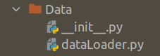
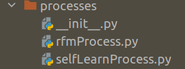


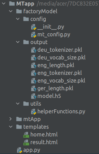
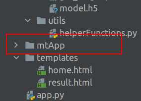


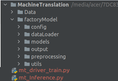
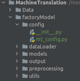


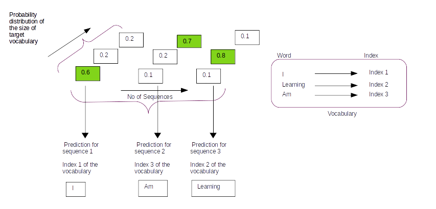


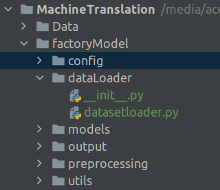
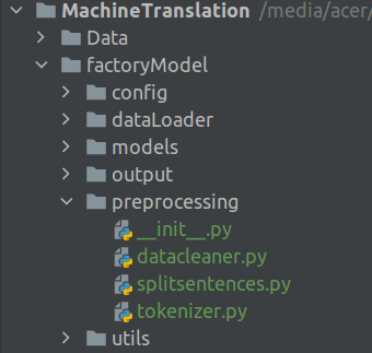
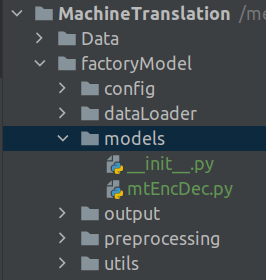


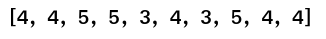


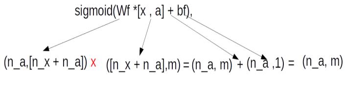
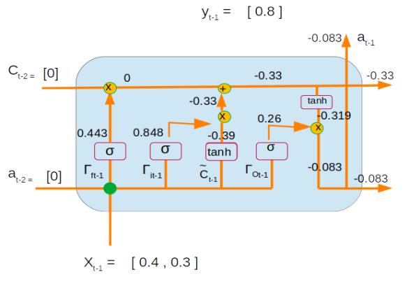

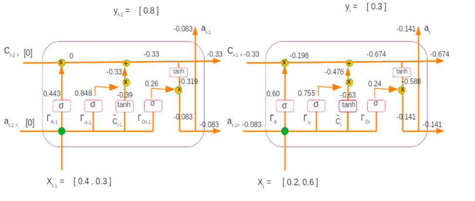

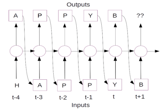
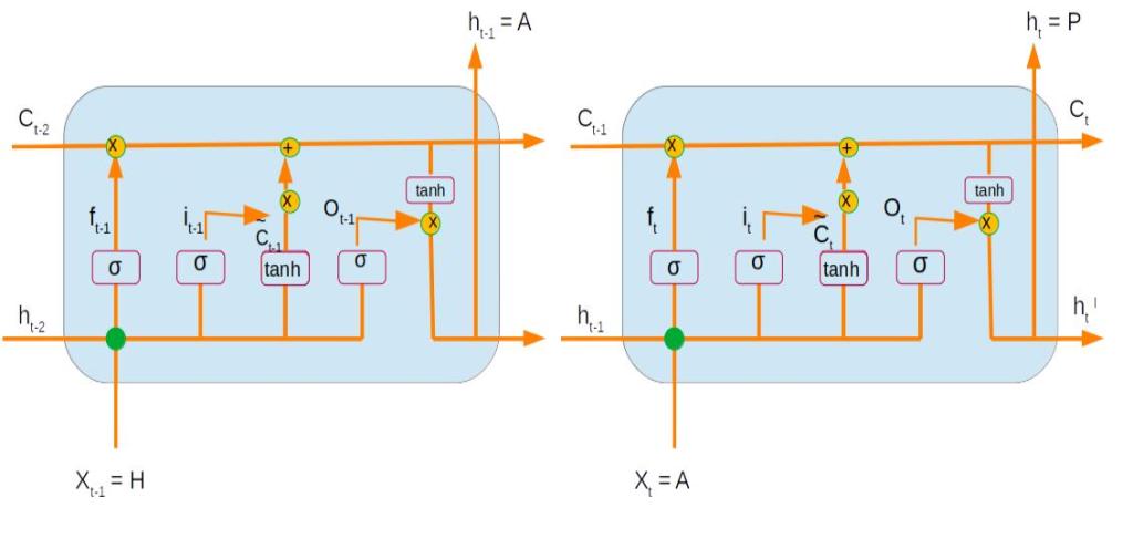


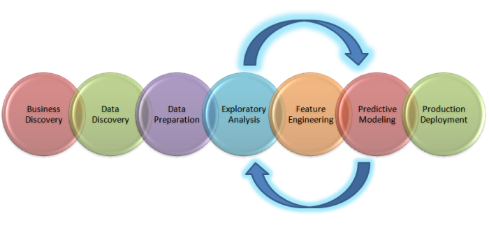
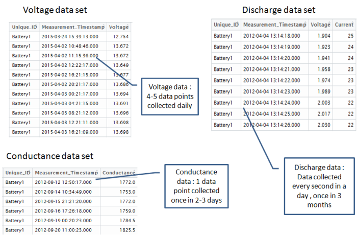


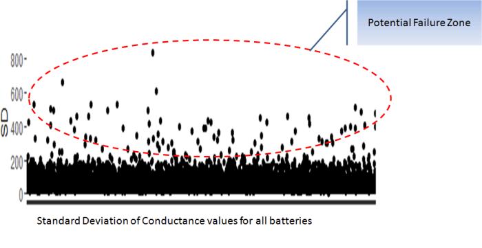
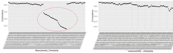

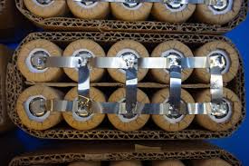
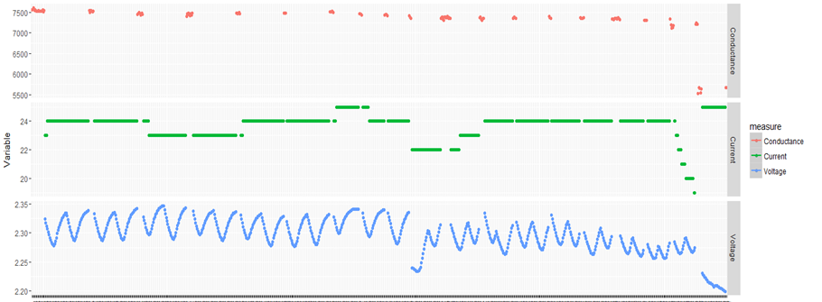

 The above is a plot depicting standard deviation of conductance for all batteries. Now what might be of interest to us is the red zone which we can call the “Potential failure Zone”. The potential failure zone consists of those batteries whose conductance values show high standard deviation. Batteries with failing health are likely to exhibit large fall in conductance and as a corollary their values will also show higher standard deviation. This implies that the samples of batteries which have higher probability of failure will in all likelihood be from this failure zone. However to ascertain this hypothesis we will have to dig deep into batteries in the failure zone and look for patterns which might differentiate them from normal batteries. Another objective to dig deep is also to elicit clues from the underlying patterns on what features to include in the predictive model. We will discuss more on the feature extraction when we discuss about feature engineering. Now let us come back to our discussion on digging deep into the failure zone and ferreting out significant patterns. It has to be noted that in addition to the samples in the failure zone we will also have to observe patterns from the normal zone to help separate wheat from the chaff . Intuitions derived by observing different patterns would become vital during feature engineering stage.