This is the sixth post of our series on building a self learning recommendation system using reinforcement learning. This series consists of 8 posts where in we progressively build a self learning recommendation system. This series consists of the following posts
- Recommendation system and reinforcement learning primer
- Introduction to multi armed bandit problem
- Self learning recommendation system as a K-armed bandit
- Build the prototype of the self learning recommendation system : Part I
- Build the prototype of the self learning recommendation system : Part II
- Productionising the self learning recommendation system: Part I – Customer Segmentation ( This post )
- Productionising the self learning recommendation system: Part II – Implementing self learning recommendation
- Evaluating different deployment options for the self learning recommendation systems.
This post builds on the previous post where we started off with building the prototype of the application in Jupyter notebooks. In this post we will see how to convert our prototype into Python scripts. Converting into python script is important because that is the basis for building an application and then deploying them for general consumption.
File Structure for the project
First let us look at the file structure of our project.

The directory RL_Recomendations is the main directory which contains other folders which are required for the project. Out of the directories rlreco is a virtual environment we will create and all our working directories are within this virtual environment.Along with the folders we also have the script rlRecoMain.py which is the main driver script for the application. We will now go through some of the steps in creating this folder structure
When building an application it is always a good practice to create a virtual environment and then complete the application build process within the virtual environment. We talked about this in one of our earlier series for building machine translation applications . This way we can ensure that only application specific libraries and packages are present when we deploy our application.
Let us first create a separate folder in our drive and then create a virtual environment within that folder. In a Linux based system, a seperate folder can be created as follows
$ mkdir RL_Recomendations
Once the new directory is created let us change directory into the RL_Recomendations directory
RL_Recomendations $ python3 -m venv rlreco
Here the rlreco is the name of our virtual environment. The virtual environment which we created can be activated as below
RL_Recomendations $ source rlreco/bin/activate
Once the virtual environment is enabled we will get the following prompt.
(rlreco) ~$
In addition you will notice that a new folder created with the same name as the virtual environment. We will use that folder to create all our folders and main files required for our application. Let us traverse through our driver file and then create all the folders and files required for our application.
Create the driver file
Open a file using your favourite editor and name it rlRecoMain.py and the insert the following code.
import argparse
import pandas as pd
from utils import Conf,helperFunctions
from Data import DataProcessor
from processes import rfmMaker,rlLearn,rlRecomend
from utils import helperFunctions
import os.path
from pymongo import MongoClient
Lines 1-2 we import the libraries which we require for our application. In line 3 we have to import Conf class from the utils folder.
So first let us create a folder called utils, which will have the following file structure.

The utils folder has a file called Conf.py which contains the Conf class and another file called helperFunctions.py . The first file controls the configuration functions and the second file contains some of the helper functions like saving data into pickle files. We will get to that in a moment.
First let us open a new python file Conf.py and copy the following code.
from json_minify import json_minify
import json

class Conf:

    def __init__(self,confPath):
        # Read the json file and load it into a dictionary
        conf = json.loads(json_minify(open(confPath).read()))
        self.__dict__.update(conf)
    def __getitem__(self, k):
        return self.__dict__.get(k,None)
The Conf class is a simple class, with its constructor loading the configuration file which is in json format in line 8. Once the configuration file is loaded the elements are extracted by invoking ‘conf’ method. We will see more of how this is used later.
We have talked about the Conf class which loads the configuration file, however we havent made the configuration file yet. As you may know a configuration file contains all the parameters in the application. Let us see the directory structure of the configuration file.

You can now create the folder called config, under the rlreco folder and then open a file in your editor and then name it custprof.json and include the following code.
{

  /****
  * paths required
  ****/

  "inputData" : "/media/acer/7DC832E057A5BDB1/JMJTL/Tomslabs/Datasets/Retail/OnlineRetail.csv",
  "custDetails" : "/media/acer/7DC832E057A5BDB1/JMJTL/Tomslabs/BayesianQuest/RL_Recomendations/rlreco/output/custDetails.pkl",

  /****
  * Column mapping
  ****/

  "order_id" : "InvoiceNo",
  "product_id": "StockCode",
  "product" : "Description",
  "prod_qnty" : "Quantity",
  "order_date" : "InvoiceDate",
  "unit_price" : "UnitPrice",
  "customer_id" : "CustomerID",
    /****
  * Parameters
  ****/

  "nclust" : 4,
  "monthPer" : 15,
  "epsilon" : 0.1,
  "nProducts" : 10,
  "buyReward" : 5,
  "clickReward": 1
}
As you can see the config, file contains all the configuration items required as part of the application. The first part is where the paths to the raw file and processed pickle files are stored. The second part is the mapping of the column names in the raw file and the names used in our application. The third part contains all the parameters required for the application. The Conf class which we earlier saw will read the json file and all these parameters will be loaded to memory for us to be used in the application.
Lets come back to the utils folder and create the second file which we will name as helperFunctions.py and insert the following code.
from pickle import load
from pickle import dump
import numpy as np


# Function to Save data to pickle form
def save_clean_data(data,filename):
    dump(data,open(filename,'wb'))
    print('Saved: %s' % filename)

# Function to load pickle data from disk
def load_files(filename):
    return load(open(filename,'rb'))
This file contains two functions. The first function starting in line 7 saves a file in pickle format to the specified path. The second function in line 12, loads a pickle file and return the data. These two functions are handy functions which will be used later in our project.
We will come back to the main file rlRecoMain.py and look at the next folder and methods on line 4. In this line we import DataProcessor method from the folder Data . Let us take a look at the folder called Data.
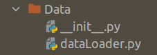
Create the data processor module
The class and the methods associated with the class are in the file dataLoader.py. Let us first create the folder, Data and then open a file named dataLoader.py and insert the following code.
import os
import pandas as pd
import pickle
import numpy as np
import random
from utils import helperFunctions
from datetime import datetime, timedelta,date
from dateutil.parser import parse

class DataProcessor:
    def __init__(self,configfile):
        # This is the first method in the DataProcessor class
        self.config = configfile

     # This is the method to load data from the input files
    def dataLoader(self):
        inputPath = self.config["inputData"]
        dataFrame = pd.read_csv(inputPath,encoding = "ISO-8859-1")
        return dataFrame

    # This is the method for parsing dates
    def dateParser(self):
        custDetails = self.dataLoader()
        #Parsing  the date
        custDetails['Parse_date'] = custDetails[self.config["order_date"]].apply(lambda x: parse(x))
        # Parsing the weekdaty
        custDetails['Weekday'] = custDetails['Parse_date'].apply(lambda x: x.weekday())
        # Parsing the Day
        custDetails['Day'] = custDetails['Parse_date'].apply(lambda x: x.strftime("%A"))
        # Parsing the Month
        custDetails['Month'] = custDetails['Parse_date'].apply(lambda x: x.strftime("%B"))
        # Getting the year
        custDetails['Year'] = custDetails['Parse_date'].apply(lambda x: x.strftime("%Y"))
        # Getting year and month together as one feature
        custDetails['year_month'] = custDetails['Year'] + "_" +custDetails['Month']

        return custDetails

    def gvCreator(self):
        custDetails = self.dateParser()
        # Creating gross value column
        custDetails['grossValue'] = custDetails[self.config["prod_qnty"]] * custDetails[self.config["unit_price"]]

        return custDetails
The constructor of the DataProcessor class takes the config file as the input and then make it available for all the other methods in line 13.
This dataProcessor class will have three methods, dataLoader, dateParser and gvCreator. The last method is the driving method which internally calls other two methods. Let us look at the gvCreator method.
The dateParser method is called first within the gvCreator method in line 40. The dateParser method in turn calls the dataLoader method in line 23. The dataLoader method loads the customer data as a pandas data frame in line 18 and the passes it to the dateParser method in line 23. The dateParser method takes the custDetails data frame and then extracts all the date related fields from lines 25-35. We saw this in detail during the prototyping phase in the previous post.
Once the dates are parsed in the custDetails data frame, it is passed to gvCreator method in line 40 and then the ‘gross value’ is calcuated by multiplying the unit price and the product quantity. Finally the processed custDetails file is returned.
Now we will come back to the rlRecoMain file and the look at the three other classes, rfmMaker,rlLearn,rlRecomend, we import in line 5 of the file rlRecoMain.py. This is imported from the ‘processes’ folder. Let us look at the composition of the processes folder.
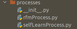
We have three files in the folder, processes.
The first one is the __init__.py file which is the constructor to the package. Let us see its contentes. Open a file and name it __init__.py and add the following lines of code.
from .rfmProcess import rfmMaker
from .selfLearnProcess import rlLearn,rlRecomend
Create customer segmentation modules
In lines 1-2 of the constructor file we make the three classes ( rfmMaker,rlLearn and rlRecomendrfmMakerrfmProcess.py and the other two classes are in the file selfLearnProcess.py.
Let us open a new file, name it rfmProcess.py and then insert the following code.
import sys
sys.path.append('path_to_the_folder/RL_Recomendations/rlreco')
import pandas as pd
import lifetimes
from sklearn.cluster import KMeans
from utils import helperFunctions


class rfmMaker:
    def __init__(self,custDetails,conf):
        self.custDetails = custDetails
        self.conf = conf

    def rfmMatrix(self):
        # Converting data to RFM format
        RfmAgeTrain = lifetimes.utils.summary_data_from_transaction_data(self.custDetails, self.conf['customer_id'], 'Parse_date','grossValue')
        # Reset the index
        RfmAgeTrain = RfmAgeTrain.reset_index()
        return RfmAgeTrain

    # Function for ordering cluster numbers

    def order_cluster(self,cluster_field_name, target_field_name, data, ascending):
        # Group the data on the clusters and summarise the target field(recency/frequency/monetary) based on the mean value
        data_new = data.groupby(cluster_field_name)[target_field_name].mean().reset_index()
        # Sort the data based on the values of the target field
        data_new = data_new.sort_values(by=target_field_name, ascending=ascending).reset_index(drop=True)
        # Create a new column called index for storing the sorted index values
        data_new['index'] = data_new.index
        # Merge the summarised data onto the original data set so that the index is mapped to the cluster
        data_final = pd.merge(data, data_new[[cluster_field_name, 'index']], on=cluster_field_name)
        # From the final data drop the cluster name as the index is the new cluster
        data_final = data_final.drop([cluster_field_name], axis=1)
        # Rename the index column to cluster name
        data_final = data_final.rename(columns={'index': cluster_field_name})
        return data_final

    # Function to do the cluster ordering for each cluster
    #

    def clusterSorter(self,target_field_name,RfmAgeTrain, ascending):
        # Defining the number of clusters
        nclust = self.conf['nclust']
        # Make the subset data frame using the required feature
        user_variable = RfmAgeTrain[['CustomerID', target_field_name]]
        # let us take four clusters indicating 4 quadrants
        kmeans = KMeans(n_clusters=nclust)
        kmeans.fit(user_variable[[target_field_name]])
        # Create the cluster field name from the target field name
        cluster_field_name = target_field_name + 'Cluster'
        # Create the clusters
        user_variable[cluster_field_name] = kmeans.predict(user_variable[[target_field_name]])
        # Sort and reset index
        user_variable.sort_values(by=target_field_name, ascending=ascending).reset_index(drop=True)
        # Sort the data frame according to cluster values
        user_variable = self.order_cluster(cluster_field_name, target_field_name, user_variable, ascending)
        return user_variable


    def clusterCreator(self):

        #data : THis is the dataframe for which we want to create the clsuters
        #clustName : This is the variable name
        #nclust ; Numvber of clusters to be created

        # Get the RFM data Frame
        RfmAgeTrain = self.rfmMatrix()
        # Implementing for user recency
        user_recency = self.clusterSorter('recency', RfmAgeTrain,False)
        #print('recency grouping',user_recency.groupby('recencyCluster')['recency'].mean().reset_index())
        # Implementing for user frequency
        user_freqency = self.clusterSorter('frequency', RfmAgeTrain, True)
        #print('frequency grouping',user_freqency.groupby('frequencyCluster')['frequency'].mean().reset_index())
        # Implementing for monetary values
        user_monetary = self.clusterSorter('monetary_value', RfmAgeTrain, True)
        #print('monetary grouping',user_monetary.groupby('monetary_valueCluster')['monetary_value'].mean().reset_index())

        # Merging the individual data frames with the main data frame
        RfmAgeTrain = pd.merge(RfmAgeTrain, user_monetary[["CustomerID", 'monetary_valueCluster']], on='CustomerID')
        RfmAgeTrain = pd.merge(RfmAgeTrain, user_freqency[["CustomerID", 'frequencyCluster']], on='CustomerID')
        RfmAgeTrain = pd.merge(RfmAgeTrain, user_recency[["CustomerID", 'recencyCluster']], on='CustomerID')
        # Calculate the overall score
        RfmAgeTrain['OverallScore'] = RfmAgeTrain['recencyCluster'] + RfmAgeTrain['frequencyCluster'] + RfmAgeTrain['monetary_valueCluster']
        return RfmAgeTrain

    def segmenter(self):

        #This is the script to create segments after the RFM analysis

        # Get the RFM data Frame
        RfmAgeTrain = self.clusterCreator()
        # Segment data
        RfmAgeTrain['Segment'] = 'Q1'
        RfmAgeTrain.loc[(RfmAgeTrain.OverallScore == 0), 'Segment'] = 'Q2'
        RfmAgeTrain.loc[(RfmAgeTrain.OverallScore == 1), 'Segment'] = 'Q2'
        RfmAgeTrain.loc[(RfmAgeTrain.OverallScore == 2), 'Segment'] = 'Q3'
        RfmAgeTrain.loc[(RfmAgeTrain.OverallScore == 4), 'Segment'] = 'Q4'
        RfmAgeTrain.loc[(RfmAgeTrain.OverallScore == 5), 'Segment'] = 'Q4'
        RfmAgeTrain.loc[(RfmAgeTrain.OverallScore == 6), 'Segment'] = 'Q4'

        # Merging the customer details with the segment
        custDetails = pd.merge(self.custDetails, RfmAgeTrain, on=['CustomerID'], how='left')
        # Saving the details as a pickle file
        helperFunctions.save_clean_data(custDetails,self.conf["custDetails"])
        print("[INFO] Saved customer details ")

        return custDetails
The rfmMaker, class contains methods which does the following tasks,Converting the custDetails data frame to the RFM format. We saw this method in the previous post, where we used the lifetimes library to convert the data frame to the RFM format. This process is detailed in the rfmMatrix method from lines 15-20.
Once the data is made in the RFM format, the next task as we saw in the previous post was to create the clusters for recency, frequency and monetary values. During our prototyping phase we decided to adopt 4 clusters for each of these variables. In this method we will pass the number of clusters through the configuration file as seen in line 44 and then we create these clusters using Kmeans method as shown in lines 48-49. Once the clusters are created, the clusters are sorted to get a logical order. We saw these steps during the prototyping phase and these are implemented using clusterCreator method ( lines 61-85) clusterSorter method ( lines 42-58 ) and orderCluster methods ( lines 24 – 37 ). As the name suggests the first method is to create the cluster and the latter two are to sort it in the logical way. The detailed explanations of these functions are detailed in the last post.
After the clusters are made and sorted, the next task was to merge it with the original data frame. This is done in the latter part of the clusterCreator method ( lines 80-82 ). As we saw in the prototyping phase we merged all the three cluster details to the original data frame and then created the overall score by summing up the scores of each of the individual clusters ( line 84 ) . Finally this data frame is returned to the final method segmenter for defining the segments
Our final task was to combine the clusters to 4 distinct segments as seen from the protoyping phase. We do these steps in the segmenter method ( lines 94-100 ). After these steps we have 4 segments ‘Q1’ to ‘Q4’ and these segments are merged to the custDetails data frame ( line 103 ).
Thats takes us to the end of this post. So let us summarise all our learning so far in this post.
- Created the folder structure for the project
- Created a virtual environment and activated the virtual environment
- Created folders like Config, Data, Processes, Utils and the created the corresponding files
- Created the code and files for data loading, data clustering and segmenting using the RFM process
We will not get into other aspects of building our self learning system in the next post.
What Next ?
Now that we have explored rfmMaker class in file rfmProcess.py in the next post we will define the classes and methods for implementing the recommendation and self learning processes. The next post will be published next week. To be notified of the next post please subscribe to this blog post .You can also subscribe to our Youtube channel for all the videos related to this series.
The complete code base for the series is in the Bayesian Quest Git hub repository
Do you want to Climb the Machine Learning Knowledge Pyramid ?
Knowledge acquisition is such a liberating experience. The more you invest in your knowledge enhacement, the more empowered you become. The best way to acquire knowledge is by practical application or learn by doing. If you are inspired by the prospect of being empowerd by practical knowledge in Machine learning, subscribe to our Youtube channel
I would also recommend two books I have co-authored. The first one is specialised in deep learning with practical hands on exercises and interactive video and audio aids for learning

This book is accessible using the following links
The Deep Learning Workshop on Amazon
The Deep Learning Workshop on Packt
The second book equips you with practical machine learning skill sets. The pedagogy is through practical interactive exercises and activities.

This book can be accessed using the following links
The Data Science Workshop on Amazon
The Data Science Workshop on Packt
Enjoy your learning experience and be empowered !!!!


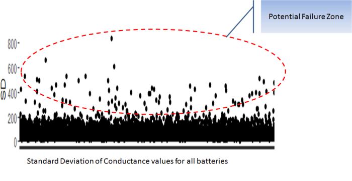
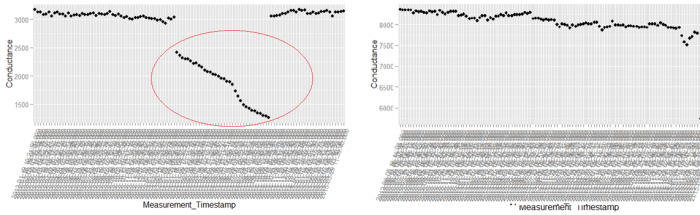


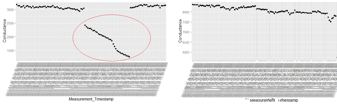
 The above is a plot depicting standard deviation of conductance for all batteries. Now what might be of interest to us is the red zone which we can call the “Potential failure Zone”. The potential failure zone consists of those batteries whose conductance values show high standard deviation. Batteries with failing health are likely to exhibit large fall in conductance and as a corollary their values will also show higher standard deviation. This implies that the samples of batteries which have higher probability of failure will in all likelihood be from this failure zone. However to ascertain this hypothesis we will have to dig deep into batteries in the failure zone and look for patterns which might differentiate them from normal batteries. Another objective to dig deep is also to elicit clues from the underlying patterns on what features to include in the predictive model. We will discuss more on the feature extraction when we discuss about feature engineering. Now let us come back to our discussion on digging deep into the failure zone and ferreting out significant patterns. It has to be noted that in addition to the samples in the failure zone we will also have to observe patterns from the normal zone to help separate wheat from the chaff . Intuitions derived by observing different patterns would become vital during feature engineering stage.