“One measure of success will be the degree to which you build up others“
This is the last post of the series and in this post we finally build and deploy our application we painstakingly developed over the past 7 posts . This series comprises of 8 posts.
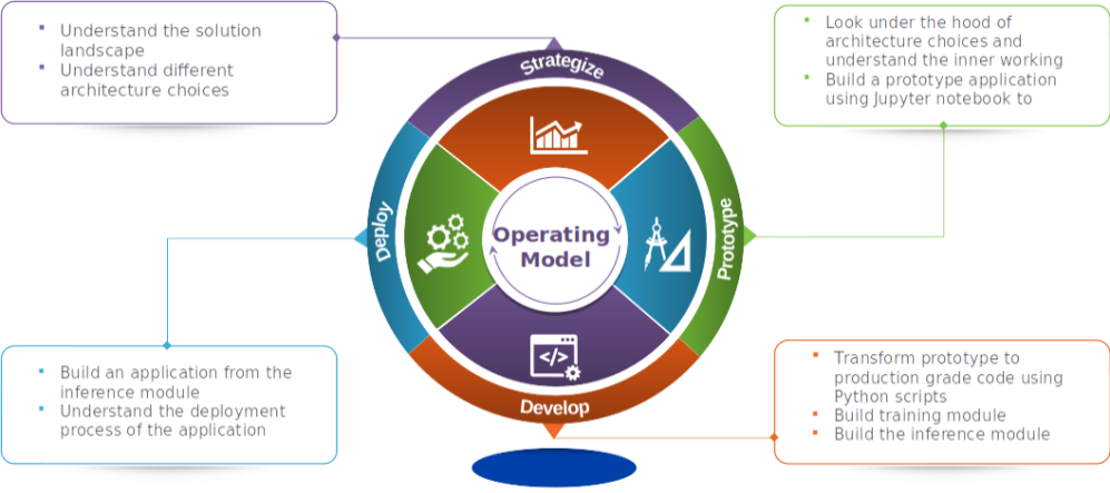
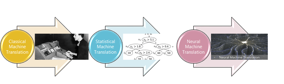
- Understand the landscape of solutions available for machine translation
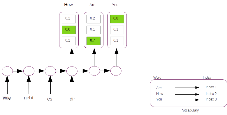
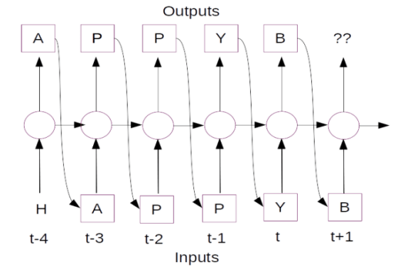
- Explore sequence to sequence model architecture for machine translation.
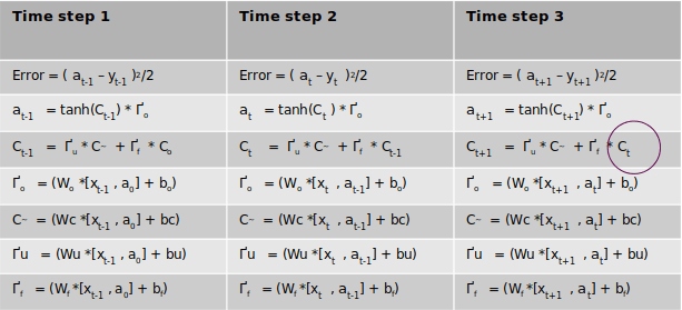
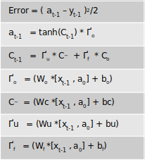
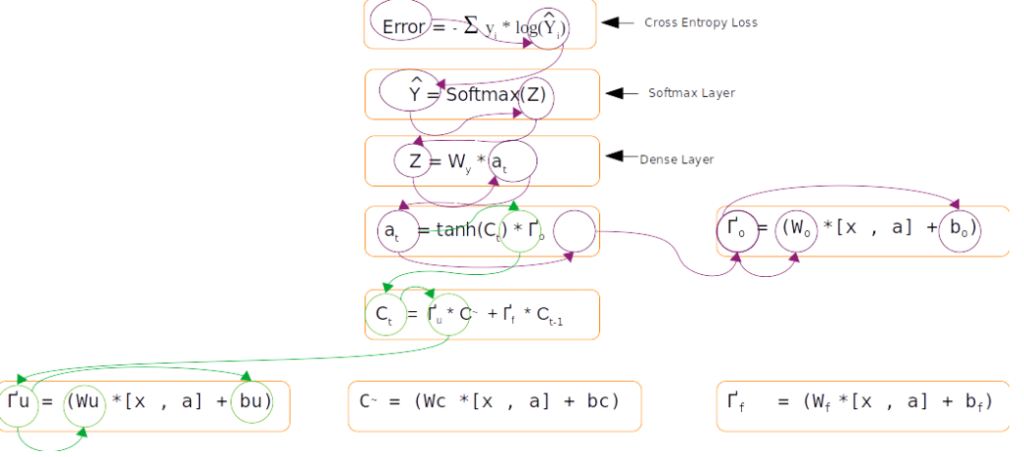
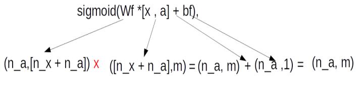
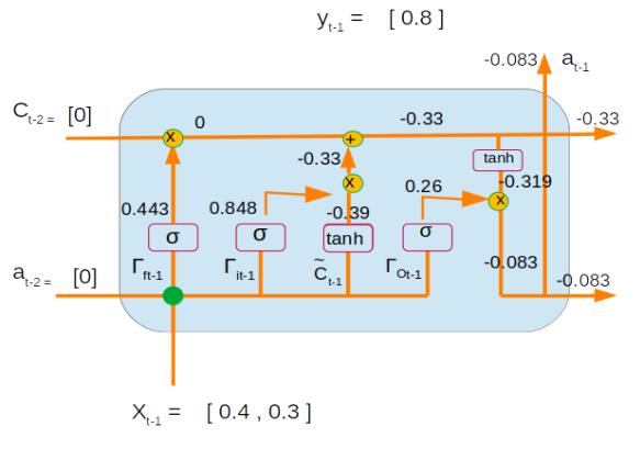
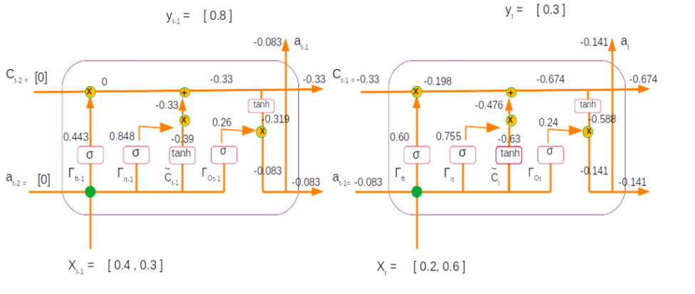
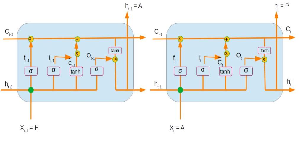
- Deep dive into the LSTM model with worked out numerical example.
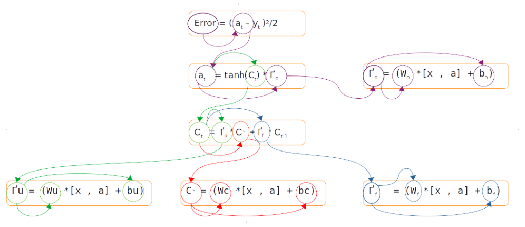
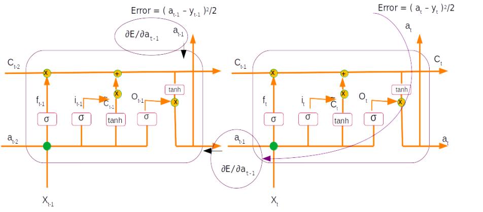
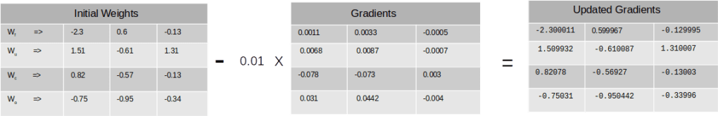
- Understand the back propagation algorithm for a LSTM model worked out with a numerical example.
- Build a prototype of the machine translation model using a Google colab / Jupyter notebook.
- Build the production grade code for the training module using Python scripts.
- Building the Machine Translation application -From Prototype to Production : Inference process
- Building the Machine Translation application: Build and deploy using Flask : ( This post)
Over the last two posts we covered the factory model and saw how we could build the model during the training phase. We also saw how the model was used for inference. In this section we will take the results of these predictions and build an app using flask. We will progressively work through the different processes of building the application.
Folder Structure
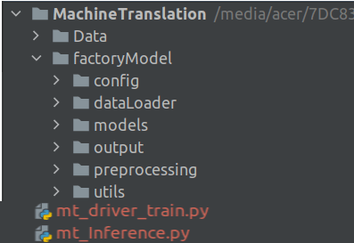
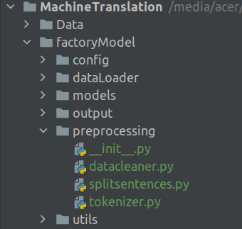
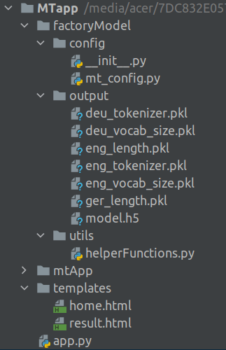
In our journey so far we progressively built many files which were required for the training phase and the inference phase. Now we are getting into the deployment phase were we want to deploy the code we have built into an application. Many of the files which we have built during the earlier phases may not be required anymore in this phase. In addition, we want the application we deploy as light as possible for its performance. For this purpose it is always a good idea to create a seperate folder structure and a new virtual environment for deploying our application. We will only select the necessary files for the deployment purpose. Our final folder structure for this phase will look as follows
Let us progressively build this folder structure and the required files for building our machine translation application.
Setting up and Installing FLASK
When building an application in FLASK , it is always a good practice to create a virtual environment and then complete the application build process within the virtual environment. This way we can ensure that only application specific libraries and packages are deployed into the hosting service. You will see later on that creating a seperate folder and a new virtual environment will be vital for deploying the application in Heroku.
Let us first create a separate folder in our drive and then create a virtual environment within that folder. In a Linux based system, a seperate folder can be created as follows
$ mkdir mtApp
Once the new directory is created let us change directory into the mtApp directory and then create a virtual environment. A virtual environment can be created on Linux with Python3 with the below script
mtApp $ python3 -m venv mtApp
Here the second mtApp is the name of our virtual environment. Do not get confused with the directory we created with the same name. The virtual environment which we created can be activated as below
mtApp $ source mtApp/bin/activate
Once the virtual environment is enabled we will get the following prompt.
(mtApp) ~$
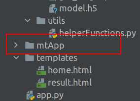
In addition you will notice that a new folder created with the same name as the virtual environment
Our next task is to install all the libraries which are required within the virtual environment we created.
(mtApp) ~$ pip install flask
(mtApp) ~$ pip install tensorflow
(mtApp) ~$ pip install gunicorn
That takes care of all the installations which are required to run our application. Let us now look through the individual folders and the files within it.
There would be three subfolders under the main application folder MTapp. The first subfolder factoryModel is a subset of the corrsponding folder we maintained during the training phase. The second subfolder mtApp is the one created when the virtual environment was created. We dont have to do anything with that folder. The third folder templates is a folder specifically for the flask application. The file app.py is the driver file for the flask application. Let us now looks into each of the folders.

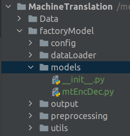
Folder 1 : factoryModel:
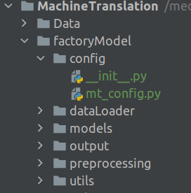
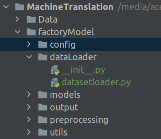
The subfolders and files under the factoryModel folder are as shown below. These subfolders and its files are the same as what we have seen during the training phase.

The config folder contains the __init__.py file and the configuration file mt_config.py we used during the training and inference phases.
The output folder contains only a subset of the complete output folder we saw during the inference phase. We need only those files which are required to translate an input German string to English string. The model file we use is the one generated after the training phase.
The utils folder has the same helperFunctions script which we used during the training and inference phase.
Folder 2 : Templates :

The templates folder has two html templates which are required to visualise the outputs from the flask application. We will talk more about the contents of the html file in a short while along with our discussions on the flask app.
Flask Application
Now its time to get to the main part of this article, which is, building the script for the flask application. The code base for the functionalities of the application will be the same as what we have seen during the inference phase. The difference would be in terms of how we use the predictions and visualise them on to the web browser using the flask application.
Let us now open a new file and name is app.py. Let us start building the code in this file
'''
This is the script for flask application
'''

from tensorflow.keras.models import load_model
from factoryModel.config import mt_config as confFile
from factoryModel.utils.helperFunctions import *
from flask import Flask,request,render_template

# Initializing the flask application
app = Flask(__name__)

## Define the file path to the model
modelPath = confFile.MODEL_PATH

# Load the model from the file path
model = load_model(modelPath)
Lines 5-8 imports the required libraries for creating the application
Lines 11 creates the application object ‘app’ as an instance of the class ‘Flask’. The (__name__) variable passed to the Flask class is a predefined variable used in Python to set the name of the module in which it is used.
Line 14 we load the configuration file from the config folder.
Line 17 The model which we created during the training phase is loaded using the load_model() function in Keras.
Next we will load the required pickle files we saved after the training process. In lines 20-22 we intialize the paths to all the files and variables we saved as pickle files during the training phase. These paths are defined in the configuration file. Once the paths are initialized the required files and variables are loaded from the respecive pickle files in lines 24-27. We use the load_files() function we defined in the helper function script for loading the pickle files. You can notice that these steps are same as the ones we used during the inference process.
In the next lines we will explore the visualisation processes for flask application.
@app.route('/')
def home():
	return render_template('home.html')
Lines 29:31 is a feature called the ‘decorator’. A decorator is used to modify the function which comes after it. The function which follows the decorator is a very simple function which returns the html template for our landing page. The landing page of the application is a simple text box where the source language (German) has to be entered. The purpose of the decorator is to build a mapping between the function and the url for the landing page. The URL’s are defined through another important component called ‘routes’ . ‘Routes’ modules are objects which configures the webpages which receives inputs and displays the returned outputs. There are two ‘routes’ which are required for this application, one corresponding to the home page (‘/’) and the second one mapping to another webpage called ‘/translate. The way the decorator, the route and the associated function works together is as follows. The decorator first defines the relationship between the function and the route. The function returns the landing page and route shows the location where the landing page has to be displayed.
Next we will explore the next decorator which return the predictions
@app.route('/translate', methods=['POST', 'GET'])
def get_translation():
    if request.method == 'POST':

        result = request.form
        # Get the German sentence from the Input site
        gerSentence = str(result['input_text'])
        # Converting the text into the required format for prediction
        # Step 1 : Converting to an array
        gerAr = [gerSentence]
        # Clean the input sentence
        cleanText = cleanInput(gerAr)
        # Step 2 : Converting to sequences and padding them
        # Encode the inputsentence as sequence of integers
        seq1 = encode_sequences(Ger_tokenizer, int(Ger_stdlen), cleanText)
        # Step 3 : Get the translation
        translation = generatePredictions(model,Eng_tokenizer,seq1)
        # prediction = model.predict(seq1,verbose=0)[0]

        return render_template('result.html', trans=translation)
Line 33. Our application is designed to accept German sentences as input, translate it to English sentences using the model we built and output the prediction back to the webpage. By default, the routes decorator only receives input i.e ‘GET’ requests. In order to return the predicted words, we have to define a new method in the decorator route called ‘POST’. This is done through the parameters methods=['POST','GET'] in the decorator.
Line 34. is the main function which translates the input German sentences to English sentences and then display the predictions on to the webpage.
Line 35, defines the ‘if’ method to ascertain that there is a ‘POST’ method which is involved in the operation. The next line is where we define the web form which is used for getting the inputs from the application. Web forms are like templates which are used for receiving inputs from the users and also returning the output.
In Line 37 we define the request.form into a new variable called result. All the outputs from the web forms will be accessible through the variable result.There are two web forms which we use in the application ‘home.html’ and ‘result.html’.
By default the webforms have to reside in a folder called Templates. Before we proceed with the rest of the code within the function we have to understand the webforms. Therefore let us build them. Open a new file and name it home.html and copy the following code.
<!DOCTYPE html>

<html>
<title>Machine Translation APP</title>
<body>
<form action = "/translate" method= "POST">

	<h3> German Sentence: </h3>

	<th> <input name='input_text' type="text" value = " " /> </th>

	<p><input type = "submit" value = "submit" /></p>

</form>
</body>
</html>
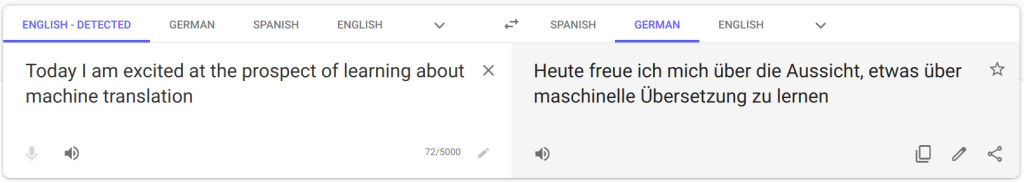
The prediction process in our application is initiated when we get the input German text from the ‘home.html’ form. In ‘home.html’ we define the variable name ( ‘input_text’ : line 10 in home.html) for getting the German text as input. A default value can also be mentioned using the variable value which will be over written when a new text is given as input. We also specify a submit button for submitting the input German sentence through the form, line 12.
Line 39 : As seen in line 37, the inputs from the web form will be stored in the variable result. Now to access the input text which is stored in a variable called ‘input_text’ within home.html, we have to call it as ‘input_text’ from the result variable ( result['input_text']. This input text is there by stored into a variable ‘gerSentence’ as a string.
Line 42 the string object we received from the earlier line is converted to a list as required during prediction process.
Line 44, we clean the input text using the cleanInput() function we import from the helperfunctions. After cleaning the text we need to convert the input text into a sequence of integers which is done in line 47. Finally in line 49, we generate the predicted English sentences.
For visualizing the translation we use the second html template result.html. Let us quickly review the template
<!DOCTYPE html>
<html>
<title>Machine Translation APP</title>

    <body>
          <h3> English Translation:  </h3>
            <tr>
                <th> {{ trans }} </th>
            </tr>
    </body>
</html>
This template is a very simple one where the only varible of interest is on line 8 which is the variable trans.
The translation generated is relayed to result.html in line 51 by assigning the translation to the parameter trans .
if __name__ == '__main__':
    app.debug = True
    app.run()
Finally to run the app, the app.run() method has to be invoked as in line 56.
Let us now execute the application on the terminal. To execute the application run $ python app.py on the terminal. Always ensure that the terminal is pointing to the virtual environment we initialized earlier.

When the command is executed you should expect to get the following screen

Click the url or copy the url on a browser to see the application you build come live on your browser.
Congratulations you have your application running on the browser. Keep entering the German sentences you want to translate and see how the application performs.
Deploying the application
You have come a long way from where you began. You have now built an application using your deep learning model. Now the next question is where to go from here. The obvious route is to deploy the application on a production server so that your application is accessible to users on the web. We have different deployment options available. Some popular ones are
- Heroku
- Google APP engine
- AWS
- Azure
- Python Anywhere …… etc.
What ever be the option you choose, deploying an application of this size will be best achieved by subscribing a paid service on any of these options. However just to go through the motions and demonstrate the process let us try to deploy the application on the free option of Heroku.
Deployment Process on Heroku
Heroku offers a free version for deployment however there are restrictions on the size of the application which can be hosted as a free service. Unfortunately our application would be much larger than the one allowed on the free version. However, here I would like to demonstrate the process of deploying the application on Heroku.
Step 1 : Creating the Heroku account.
The first step in the process is to create an account with Heroku. This can be done through the link https://www.heroku.com/. Once an account is created we get access to a dashboard which lists all the applications which we host in the platform.
Step 2 : Configuring git
Configuring ‘git’ is vital for deploying applications to Heroku. Git has to be installed first to our local system to make the deployment work. Git can be installed by following instructions in the link https://git-scm.com/book/en/v2/Getting-Started-Installing-Git.
Once ‘git’ is installed it has to be configured with your user name and email id.
$ git config –global user.name “user.name”
$ git config –global user.email userName@mail.com
Step 3 : Installing Heroku CLI
The next step is to install the Heroku CLI and the logging in to the Heroku CLI. The detailed steps which are involved for installing the Heroku CLI are given in this link
https://devcenter.heroku.com/articles/heroku-cli
If you are using Ubantu system you can install Heroku CLI using the script below
$ sudo snap install heroku --classic
Once Heroku is installed we need to log into the CLI once. This is done in the terminal with the following command
$ heroku login
Step 4 : Creating the Procfile and requirements.txt
There is a file called ‘Procfile’ in the root folder of the application which gives instructions on starting the application.

The file can be created using any text editor and should be saved in the name ‘Procfile’. No extension should be specified for the file. The contents of the file should be as follows
web: gunicorn app:app --log-file
Another important pre-requisite for the Heroku application is a file called ‘requirements.txt’. This is a file which lists down all the dependencies which needs to be installed for running the application. The requirements.txt file can be created using the below command.
$ pip freeze > requirements.txt
Step 5 : Initializing git and copying the required dependent files to Heroku
The above steps creates the basic files which are required for running the application. The next task is to initialize git on the folder. To initialize git we need to go into the root folder where the app.py file exists and then initialize it with the below command
$ git init
Step 6 : Create application instance in Heroku
In order for git to push the application file to the remote Heroku server, an instance of the application needs to be created in Heroku. The command for creating the application instance is as shown below.
$ heroku create {application name}
Please replace the braces with the application name of your choice. For example if the application name you choose is 'gerengtran', it has to be enabled as follows
$ heroku create gerengtran
Step 7 : Pushing the application files to remote server
Once git is initialized and an instance of the application is created in Heroku, the application files can be set up in remote Heroku server by the following commands.
$ heroku git:remote -a {application name}
Please note that ‘application_name’ is the name of the application which you have chosen earlier. What ever name you choose will be the name of the application in Heroku. The external link to your application will be in the name which you choose here.
Step 8 : Deploying the application and making it available as a web app
The final step of the process is to complete the deployment on Heroku and making the application available as a web app. This process starts with the command to add all the changes which you made to git.
$ git add .
Please note that there is a full stop( ‘.’ ) as part of the script after ‘add’ with a space in between .
After adding all the changes, we need to commit all the changes before finally deploying the application.
$ git commit -am "First submission"
The deployment will be completed with the below script after which the application will be up and running as a web app.
$ git push heroku master
When the files are pushed, if the deployment is successful you will get a url which is the link to the application. Alternatively, you can also go to Heroku console and activate your application. Below is the view of your console with all the applications listed. The application with the red box is the application which has been deployed

If you click on the link of the application ( red box) you get the link where the application can be open.
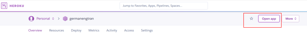
When the open app button is clicked the application is opened in a browser.
Wrapping up the series
With this we have achieved a good milestone of building an application and deploying it on the web for others to consume. I am a strong believer that learning data science should be to enrich products and services. And the best way to learn how to enrich products and services is to build it yourselves at a smaller scale. I hope you would have gained a lot of confidence by building your application and then deploying them on the web. Before we bid adeau, to this series let us summarise what we have achieved in this series and list of the next steps
In this series we first understood the solution landscape of machine translation applications and then understood different architecture choices. In the third and fourth posts we dived into the mathematics of a LSTM model where we worked out a toy example for deriving the forward pass and backpropagation. In the subsequent posts we got down to the tasks of building our application. First we built a prototype and then converted it into production grade code. Finally we wrapped the functionalities we developed in a Flask application and understood the process of deploying it on Heroku.
You have definitely come a long way.
However looking back are there avenues for improvement ? Absolutely !!!
First of all the model we built is a simple one. Machine translation is a complex process which requires lot more sophisticated models for better results. Some of the model choices you can try out are the following
- Change the model architecture. Experiment with different number of units and number of layers. Try variations like bidirectional LSTM
- Use attention mechanisms on the LSTM layers. Attention mechanism is see to have given good performance on machine translation tasks
- Move away from sequence to sequence models and use state of the art models like Transformers.
The second set of optimizations you can try out are on the vizualisations of the flask application. The templates which are used here are very basic templates. You can further experiment with different templates and make the application visually attractive.
The final improvement areas are in the choices of deployment platforms. I would urge you to try out other deployment choices and let me know the results.
I hope all of you enjoyed this series. I definitely enjoyed writing this post. Hope it benefits you and enable you to improve upon the methods used here.
I will be back again with more practical application building series like this. Watch this space for more
You can download the code for the deployment process from the following link
https://github.com/BayesianQuest/MachineTranslation/tree/master/Deployment/MTapp
Do you want to Climb the Machine Learning Knowledge Pyramid ?
Knowledge acquisition is such a liberating experience. The more you invest in your knowledge enhacement, the more empowered you become. The best way to acquire knowledge is by practical application or learn by doing. If you are inspired by the prospect of being empowerd by practical knowledge in Machine learning, I would recommend two books I have co-authored. The first one is specialised in deep learning with practical hands on exercises and interactive video and audio aids for learning

This book is accessible using the following links
The Deep Learning Workshop on Amazon
The Deep Learning Workshop on Packt
The second book equips you with practical machine learning skill sets. The pedagogy is through practical interactive exercises and activities.

This book can be accessed using the following links
The Data Science Workshop on Amazon
The Data Science Workshop on Packt
Enjoy your learning experience and be empowered !!!!