This is the second post of the series were we build a road sign and pothole detection application. We will be using multiple methods through out this series which includes computer vision techniques using opencv, annotating images using labelImg, mastering Tensorflow object detection API, Training objection detection using transfer learning, Object detection on video etc. This series will be split across 8 posts.
1. Introduction to object detection
2. Data set preperation and annotation Using labelImg ( This Post )
3. Building your road pothole detector from scratch using Image pyramids and Sliding window
4. Building your road pothole detector using RCNN
5. Building your road pothole detector using YOLO
6. Building you road pothole detector using Tensorflow object detection API
7. Building your video analytics application for detecting potholes
8. Deploying your video analytics application for detection of potholes
In this post we will talk about the data annotation and data preperation stage of the process
Data Sets for Object Detection
In the last post we got introduced to Object detection tasks. We also briefly discovered some of the leading approaches for object detection. When discussing about model training approaches you would have identified that the data sets for object detection are not exactly like any data sets which you would have encountered in your normal machine learning lifecycle. Object detection data sets have two sets of labels, one is the class label for the objects and the second is the bounding boxes for each of the object. The bounding boxes contains the (x ,y )cordinates of the four corners where the object is present. There are different publicly available data sets for object detection tasks. The coco dataset being one of the most popular ones
For the specific task which we are dealing with i.e. Pothole detection, we might not have annotated data sets. Therefore we will have to create that dataset which includes the class labels and the bounding boxes.
This post will talk about downloading data for pothole detection, creating the class labels and bounding boxes for the data and then extracting the necessary information from the annotation task so that we can use it for training the data set. In this exercise we will use a tool called labelIMG which will be used for annotating the dataset.
Installing and Configuraing labelIMG
LabelImg is a free, open source tool for graphically labeling images. It’s written in Python and is an easy, free way to label images for your object detection projects.
Installation of labelImg is quite simple and it can be installed using pip command for python3 as shown below.
pip3 install labelImg
To know more about the installation and configuration you can refer the following link.
Lets now look at how we collect data and annotate them using labelImg
Raw Data Creation
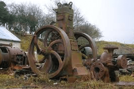
The first task is to create the data set required for training the model and also annotation. The images which are used in this series are collected from google images.
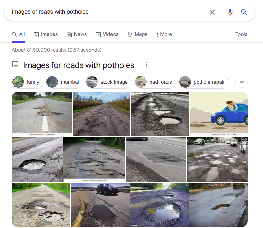
You can download as many images as you want for this task. Always remember to get some good variety of images with different type of objects which you are likely to see on roads.
Annotation of the images
The annotation of the images are done using labelImg application.
To activate the labelImg application, just invoke the labelImg command on the terminal as follows

Once this is activated a front end will be opened as follows

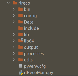
We start with selecting the directory where the files are stored. We select the directory using the open Dir icon. Once we select the Open Dir icon we will get all the images in the direcotry listed in the application as follows

We navigate one image at a time, and then draw the bounding boxes of the objects we want to annotate. Once the bounding boxes are drawn we can input the label we want to give to the image. Once the bounding boxes are selected and annotation are done, the image can be saved as an xml file.

Let us open one fo the xml files and look at the information contained in the xml file. The xml file contains the bounding boxes and the class information of the images as shown below.

We have now annotated all the files with the class names and bounding boxes. Let us now extract the information from the xml files into a csv files
Extracting the Information from annotation
In this section we will extract all the annotation information into a pandas data frame and later on to csv file. We will start with importing all the library files we require.
import os
import glob
import pandas as pd
import xml.etree.ElementTree as ET
Next let us list down all the ‘xml’files in the folder using glob() method. We have to give the path of the folder where all the xml files are stored.
# Define the path
path = 'data'
# Get the list of all files in the folder
allFiles = glob.glob(path + '/*.xml')
allFiles
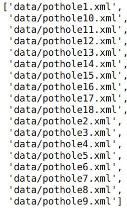
Next we need to parse through the 'xml'files and then extract the information from the file. We will use the 'ElementTree' method in the xml package to parse through the folder and then get the relevant information.
# Get one of the files
xml_file = allFiles[0]
# Parse xml file and get the root
tree = ET.parse(xml_file)
root = tree.getroot()
# For each element of the root print the tag and the attribute
for child in root:
    print(child.tag, child.attrib)

In line 13 -14 we get the 'tree' object and the get the 'root' of the xml file. The root contains all the elements as children. Lines 16-17 we go through each of the elements of the xml file and then extract the tags and the attribute of the element. We can see the major elements printed. If we look at the raw xml file we can see all these elements listed there.
As seen in the output, elements named as ‘object’ are the bounding boxes we annotated in the earlier step. These objects contains the bounding box information we need. Before we extract the bounding box information, let us look at some basic methods to extract any information from the root.
filename = root.find('filename').text
filename

In line 18 we extract the filename of this xml file using the root.find() method. We need to specify which element we want to look into, which in our case is the text called ‘filename‘ as that is how it is represented in the xml file. To get the filename as a string we give the .text extension.
Let us now get the width and height of the image. We can see from the xml file that this is contained in the element, 'size'
# Extract width and height of the image
width = int(root.find('size').find('width').text)
height = int(root.find('size').find('height').text)
print(width,height)
In lines 21-22 use the find() method to extract width and height and then convert the text into integer.
Our next task is to extract the class names and the bounding box elements. These are contained in each of the 'object' elements under the name 'bndbox'. The class label of the image is contained inside this element under the element name 'name' and the bounding boxes are with the element names 'xmin','ymin','xmax','ymax'. Let us look at one of the sample object elements.
# Get all the 'object' elements
members = root.findall('object')
# Take the first one to extract the information as an example
member = members[0]
print(member.find('name').text)
print(member.find('bndbox').find('xmin').text)

From lines 28-29 we can see the class name and one of the bounding box values extracted using the find() method as seen before
Now that we have seen all the moving parts , let us encapsulate all these into a function and extract all the information into a pandas dataframe. This code is taken from this tutorial link for object detection.
def xml_to_pd(path):
    """Iterates through all .xml files (generated by labelImg) in a given directory and combines
    them in a single Pandas dataframe.

    Parameters:
    ----------
    path : str
        The path containing the .xml files
    Returns
    -------
    Pandas DataFrame
        The produced dataframe
    """

    xml_list = []
    # List down all the files within the path
    for xml_file in glob.glob(path + '/*.xml'):
        # Get the tree and the root of the xml files
        tree = ET.parse(xml_file)
        root = tree.getroot()
        # Get the filename, width and height from the respective elements
        filename = root.find('filename').text
        width = int(root.find('size').find('width').text)
        height = int(root.find('size').find('height').text)
        # Extract the class names and the bounding boxes of the classes
        for member in root.findall('object'):
            bndbox = member.find('bndbox')
            value = (filename,
                     width,
                     height,
                     member.find('name').text,
                     int(bndbox.find('xmin').text),
                     int(bndbox.find('ymin').text),
                     int(bndbox.find('xmax').text),
                     int(bndbox.find('ymax').text),
                     )
            xml_list.append(value)
    # Consolidate all the information into a data frame
    column_name = ['filename', 'width', 'height',
                   'class', 'xmin', 'ymin', 'xmax', 'ymax']
    xml_df = pd.DataFrame(xml_list, columns=column_name)
    return xml_df
Let us now extract the information of all the xml files and then convert it into a pandas data frame.
pothole_df = xml_to_pd(path)
pothole_df

Finally let us save this label information in a csv file as we will use it later for training our object detection elements.
pothole_df.to_csv('pothole_df.csv',index=False)
Having prepared the data set, let us now look at the next process which is to prepare the train and test sets.
Preparing the Training and test sets
The process of building the train images, involves multiple processes. Let us look at each of them
Mixing positive and negative images
We just annotated the images with potholes along with its bounding boxes. We will be using those images for building the positive classes for the object detector. Along with the positive classes, we also need to get some negative examples. For negative examples we will take some examples of roads without potholes. We will keep both the positive and negative examples, in seperate folders and then use them for building the training data. We will also use some augmentation techniques to increase the training data. Let us dive deeper with the preperation of the training data set.
import os
import glob
import pandas as pd
import io
import cv2
from skimage import feature
import skimage
from sklearn.feature_extraction.image import extract_patches_2d
from sklearn.svm import SVC
import numpy as np
import argparse
import pickle
import matplotlib.pyplot as plt
from random import sample
%matplotlib inline
We will start by importing all the required packages. Next let us look at the positive examples, which are the images with potholes that were downloaded in the last post.
# Positive Images
path = 'data'
allFiles = glob.glob(path + '/*.jpeg')
print(len(allFiles))
allFiles


The above figure lists the images which were downloaded and annotated earlier. You are free to download any number of images. The more the better, as the classifier will perform well with more examples. Later on we will see how we augment these images with different augmentation techniques to increase the number of positive images. However whatever the type of augmentation techniques we use, it would still not be a substitute for variety of positive images.
Let us now look at the negative classes of images. For negative classes we will be using images of normal roads. Let us look at some of the examples of the negative images
# Negative images
path = 'data/Annotated'
roadFiles = glob.glob(path + '/*.jpeg')
for imgPath in roadFiles[:2]:
    img = cv2.imread(imgPath)
    plt.imshow(img)
    plt.show()


These negative images were downloaded in the same way the positive images were also downloaded i.e. from Google images. Again more the examples the better. However what needs to be noted is to maintain a fair balance between the positive and negative examples.
Extracting HOG features from the images
Once the positive and negative images are collected, its now the turn to extract features from the images. There a different methods to extract features from images. The method we will be using is the HOG features. HOG stands for ‘Histogram of Oriented Gradients’. Let us quickly take a quick tour of the HOG method.
Histogram of Oriented Gradients ( HOG )
HOG descriptors are used to represent the structure and appearence of the object in an image. This algorithm works on the principle that an object in an image can be modeled by the distribution of intensity gradients within regions where the object reside. The implementation of this method entails dividing an image into small cells and then for each cell computing the histogram of oriented gradients for pixels within each cell. The histograms accross multiple cells are accumulated to form the feature vector. The dimensionality of these feature vectors depend on the dimension of the image and the parameters of the HOG descriptor like pixels_per_cell, cells_per_block and orientations. You can refer to the following link to learn more about HOG descriptors
Let us now implement the methods for extracting the features and saving the data set on to disk. As a first step we will read the positive images which are the pothole images. We will read the data from the information in the csv file we created earlier. We will take the information and then extract only those patches which contain potholes. Let us first look at the csv file containing the data.
# Reading the csv file
pothole_df = pd.read_csv('pothole_df.csv')
pothole_df

As seen from the output, the data set extracted here contains only 65 rows which comprises of all the classes including vegetation, signs, potholes etc. From this csv file, we will extract only the pothole data. The number of images have been kept intentionally low, so that we can also explore some augmentation techniques so as to enhance the data set. When you embark on custom solutions where data sets are not available you will have to resort to different augmentation techniques to improve your results.
Let us now exlore the dimensions of the set of potholes images we have, and then look at the average width and height of the bounding boxes. This, as we will see later, is to define the width of the window for the pyramid and sliding window techniques. We will use pothole_df data frame to find the dimensions.
# Find the mean of the x dim and y dimensions of the pothole class
xdim = np.mean(pothole_df[pothole_df['class']=='pothole']['xmax'] - pothole_df[pothole_df['class']=='pothole']['xmin'])
ydim = np.mean(pothole_df[pothole_df['class']=='pothole']['ymax'] - pothole_df[pothole_df['class']=='pothole']['ymin'])
print(xdim,ydim)

We will round off the dimensions to [80,40] which we will adopt as the window dimensions for the pyramid and sliding window methods.
# We will take the windows dimension as these dimensions rounded off
winDim = [80,40]
Once the images are read from the excel sheet, its time to extract the patches of potholes which we require, from the images. There are two functions which we require to extract the features which we want. The first one is to extract the hog features from the image. Let us look at that function first.
# Defining the hog structure
def hogFeatures(image,orientations,pixelsPerCell,cellsPerBlock,normalize=True):
    # Extracting the hog features from the image
    feat = feature.hog(image, orientations=orientations, pixels_per_cell=pixelsPerCell,cells_per_block = cellsPerBlock, transform_sqrt = normalize, block_norm="L1")
    feat[feat < 0] = 0
    return feat
The inputs to this function are the images from which we want to extract the features, the orientations, pixels per cell, cells per block and the normalize flag.
In line 40, we extract the features using feature.hog() method from the image. We provide all our parameters to the method to get the features. Once we extract the features, we remove all the negative pixels by making them as 0 in line 41. The extracted features are then returned by the function in the last line.
The next method we will see is the one to augment our images. There are different types of augmentation techniques which are useful. We will be using techniques like flipping ( both horizontal and vertical flipping) and then rotating them to diffrent angles. Let us see the function to augment our images.
# Defining the function for image augmentation
def imgAug(roi,ht,wd,extensive=True):
    # Initialise the empty list to store images
    rois = []
    # resize the ROI to the desired size
    roi = cv2.resize(roi, (ht,wd), interpolation=cv2.INTER_AREA)
    # Append the different images
    rois.append(roi)
    # Augment the image by flipping both horizontally and vertically
    rois.append(cv2.flip(roi, 1))
    if extensive:
        rois.append(cv2.flip(roi, 0))
        rois.append(cv2.rotate(roi, cv2.ROTATE_90_CLOCKWISE))
        rois.append(cv2.rotate(roi, cv2.ROTATE_90_COUNTERCLOCKWISE))
        # Rotate to other angles
        for rot in [15,45,60,75,85]:
            # Get the rotation matrix
            rotMatrix = cv2.getRotationMatrix2D((ht/2,wd/2),rot,1)
            # ROtate the matrix using the rotation matrix
            rois.append(cv2.warpAffine(roi,rotMatrix,(ht,wd)))
    return rois
The inputs to the function are the patch of image we want to augment along with the dimensions we want to resize the image. We also define a parameter called extensive to check if we want to do all the methods or just a simple horizontal flipping.
We first initialise a list to store all the augmented images in line 46 and then we go ahead and resize the image in line 48. The resized image is then appended to the list in line 50.
The first augmentation technique is implemented in the line 52 where in we flip it horizontally. The parameter 1 stands for flipping along the y axis.
Now if we want to go for extensive augmentation, we proceed with other types of augmentation. The first of these methods are the vertical flip, clockwise rotation and anticlockwise rotations as shown in lines 54-56.
Then we do 5 different rotations based on the list of angles we have specified in line 58. You can try out with more angles of your choice. To do the rotation we first have to define a rotation matrix which is centred along the centre of the image as shown in line 60. We also provide the centre of the image the angle by which we have to rotate and the scaling function as input parameters . We have chosen a scale of 1. You can try different scaling parameters and then see its effect on the image.
Once the rotation matrix is defined, the image is rotated using the method cv2.warpAffine() in line 62. Here we give the patch of image, the rotation matrix and the dimensions of the image as inputs.
We finally append all the augmented images into the list and then return the rois.
The overall process to extract the features consists of two functions as given below.
# Functions to extract the bounding boxes and the hog features
def roiExtractor(row,path):
    img = cv2.imread(path + row['filename'])
    # Get the bounding box elements
    bb = [int(row['xmin']),int(row['ymin']),int(row['xmax']),int(row['ymax'])]
    # Crop the image
    roi = img[bb[1]:bb[3], bb[0]:bb[2]]
    # Get the list of augmented images
    rois = imgAug(roi,80,40)
    return rois

def featExtractor(rois,data,labels,positive=True):
    for roi in rois:
        # Extract hog features
        feat = hogFeatures(roi,orientations,pixelsPerCell,cellsPerBlock,normalize=True)
        # Append data and labels
        data.append(feat)
        labels.append(int(1))
    return data,labels
The first of these functions is to read an image based on the information from the csv file and then crop the image based on the bounding box coordinates as shown in lines 66-70. Finally in line 72, we do the augmetation of the cropped image.
The second function takes the augmented images derived using the first function and extract the HOG features from each of them. We append the features in the list data and the labels are appended to 1 as these are the positive examples.
Having seen all the functions let us now see the process of preparing the data sets.
# Extracting pothole patches from the data
path = 'data/'
# Parameters for extracting HOG features
orientations=12
pixelsPerCell=(4, 4)
cellsPerBlock=(2, 2)
# Empty lists to store data and labels
data = []
labels = []
# Looping through the excel sheet rows
for idx, row in pothole_df.iterrows():
    if row['class'] == 'pothole':
        rois = roiExtractor(row,path)
        data,labels = featExtractor(rois,data,labels)
The process is quite straighforward. In lines 86-88, we define the parameters for HOG feature extraction. Then we initialise two empty lists in lines 90-91 to store data and the labels. We then loop through each of the rows of the pothole data frame and the extract the rois and features if the class of the row is ‘pothole’.
That was the positive examples we saw. Its now the turn of extracting features for the negative examples. Let us first list all the negative examples
# Listing all the negative examples
path = 'data/Annotated'
roadFiles = glob.glob(path + '/*.jpeg')
roadFiles

# Looping through the files
for row in roadFiles:
    # Read the image
    img = cv2.imread(row)
    # Extract patches
    patches = extract_patches_2d(img,(80,40),max_patches=10)
    # For each patch do the augmentation
    for patch in patches:
        # Get the list of augmented images
        rois = imgAug(patch,80,40,False)
        # Extract the features using HOG
        for roi in rois:
            feat = hogFeatures(roi,orientations,pixelsPerCell,cellsPerBlock,normalize=True)
            data.append(feat)
            labels.append(int(-1))
In the process for extracting negative examples , we first iterate through the files and then read each file. Since we dont have to crop a specific area within the image, we will adopt a different strategy to augment images. We extract certain patches of a fixed window size from the image. This is implemented through a method extract_patches_2d() in Sklearn. The dimension of the window size is based on the dimensions we fixed earlier. We also specify the number of patches we want to extract in line 106. For each of the patch we extract, we do only horizontal flip as it wouldnt make sense to do any other augmentation steps for the images of roads. We then extract the HOG features in line 113 like what we did for the positive examples. The labels for these examples are -1 as this is the negative image.
Having extracted features and the labels, we will now write the data to disk using h5py format.
import h5py
import numpy as np
# Define the output path
outputPath = 'data/pothole_features_all.hdf5'
# Create the database and write method
db = h5py.File(outputPath, "w")
dataset = db.create_dataset('pothole_features_all', (len(data), len(data[0]) + 1), dtype="float")
dataset[0:len(data)] = np.c_[labels, data]
db.close()
In this implementation we first define the outputPath and then create the database using the ‘write’ method. To create the dataset we use the create_dataset() method giving the name and the dimensions of the dataset. We increase the second dimenstion with +1 as we will be storing the label also in the same dataset. We finally store the dataset as numpy array where the labels and data are concatenated using the np.c_ method of numpy. After this step the new data base will get created in the specified path.
We can read the database using the h5py.File() method. Let us look at the name of the data set we earlier gave by taking the keys() of the database
# Read the h5py file
db = h5py.File(outputPath)
list(db.keys())

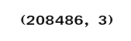
# Shape of the data
db["pothole_features_all"].shape

You can see that the shape of the data set we created. We had 730 examples of both the positive and negative examples . We can also see that we have 8209 features, which is a combination of label + the hog features of 8208.
That takes us to the end of the data preperation stage for building our object detector. In the next post we will take this data and build our object detector from scratch.
What Next ?
In the next post, we will explore different techniques to build our custom object detector. We will be covering the following topics in the next post
- Building a classifier using the training data
- Introduce the concept of Image pyramids and sliding windows
- Using Image pyramids and sliding windows to extract bouding boxes for your images
- Use non maxima suppression to eliminate overlap of bounding boxes.
We will be covering lot of ground in the next post. The next post will be published next week. To be notified of the next post please subscribe to this blog post .You can also subscribe to our Youtube channel for all the videos related to this series.
You can also access the code base for this series from the following git hub link
Do you want to Climb the Machine Learning Knowledge Pyramid ?
Knowledge acquisition is such a liberating experience. The more you invest in your knowledge enhacement, the more empowered you become. The best way to acquire knowledge is by practical application or learn by doing. If you are inspired by the prospect of being empowerd by practical knowledge in Machine learning, subscribe to our Youtube channel
I would also recommend two books I have co-authored. The first one is specialised in deep learning with practical hands on exercises and interactive video and audio aids for learning

This book is accessible using the following links
The Deep Learning Workshop on Amazon
The Deep Learning Workshop on Packt
The second book equips you with practical machine learning skill sets. The pedagogy is through practical interactive exercises and activities.

This book can be accessed using the following links
The Data Science Workshop on Amazon
The Data Science Workshop on Packt
Enjoy your learning experience and be empowered !!!!