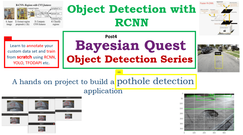
Build you computer vision application IV : Building the pothole detector using RCNN

This is the fourth post of the series were we build a pothole detection application. We will be using multiple methods on computer vision which includes annotating images using labelImg, learning about object detection and localisation, mastering Tensorflow object detection API, Training objection detection using transfer learning, Object detection on video etc. This series will be split across 8 posts.

1. Introduction to object detection

2. Data set preperation and annotation Using labelImg

3. Building your object detection model from scratch using Image pyramids and sliding window

4. Building your road pothole detector using RCNN ( This Post )

5. Building your road pothole detector using YOLO

6. Building you road pothole detector using Tensorflow object detection API

7. Building your video analytics application for detecting potholes

8. Deploying your video analytics application for detection of potholes

In the last post we built an object detector from scratch using image pyramids and sliding window techniques. These techniques are legacy techniques, however important, as these techniques lay the foundation to some of the advanced techniques. In this post we will make our foray into an advanced technique by learning about the RCNN family and then will implement an object detector using RCNN. Let us dive in.

RCNN family of object detectors

RCNN framework was originally introduced by Girshik et al. in 2013. There have been several modifications to the original architecture, resulting in better performance over time. For some time the RCNN framework was the go to model for object detection tasks.

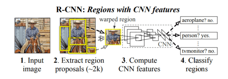
Image Source : https://arxiv.org/pdf/1311.2524.pdf

The original RCNN algorithm contains the following key steps

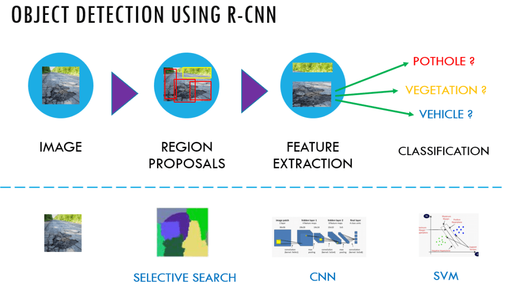
Extract regions which potentially contain an object from the input image. Such extractions are called region proposal extractions. The extractions are done using an algorithm like selective search.
Use a pretrained CNN to extract features from the proposal regions.
Classify each extracted region, using a classifier like Support Vector Machines ( SVM).

The original RCNN algorithm gave much better results than traditional methods like the sliding window and pyramid based methods. However this system was slow. Besides, deep learning was not used for localising the objects in the image and it was mostly left to algorithms like selective search.

A significant improvement was made to the original RCNN algorithm, by the same author, within a year of publishing the original paper. This algorithm was named Fast-RCNN. In this algorithm there were some novel ideas like Region of Interest Pooling layer. The Fast-RCNN algorithm used a CNN for the entire image to extract feature map from it. The region proposals were done on the feature maps extracted from the CNN layer and like the RCNN, this algorithm also used selective search for Region Proposal. A fixed size window from the feature map was extracted and then passed to a fully connected layer to get the output label for the proposal regions. This step was termed as the Region of Interest Pooling. Two sets of fully connected layers were used to get class labels of the regions along with the location of the bounding boxes for each region.

Within couple of months from the publishing of the Fast-RCNN algorithm another algorithm called the Faster-RCNN was published which improved upon the Fast-RCNN algorithm.

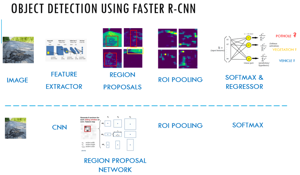
The new algorithm had another salient feature called the Region Proposal Network ( RPN), which was introduced to eliminate the need of selective search algorithm and build the capability for region proposal into the R-CNN architecture itself. In this algorithm, anchors were placed uniformly accross the entire image at varying scale and aspect ratios.

The image is split into equally spaced points called the anchor points and at each of the anchor point, 9 different anchors are generated and the Intersection over Union ( IOU ) of the anchors with the ground truth bounding boxes is determined to generate an objectness score. The objectness score is an indicator as to whether there is an object or not.

The objectness score is also used to filter down the number of proposals which will thereby be propogated to the subsequent binary classification and bounding box regression layer.

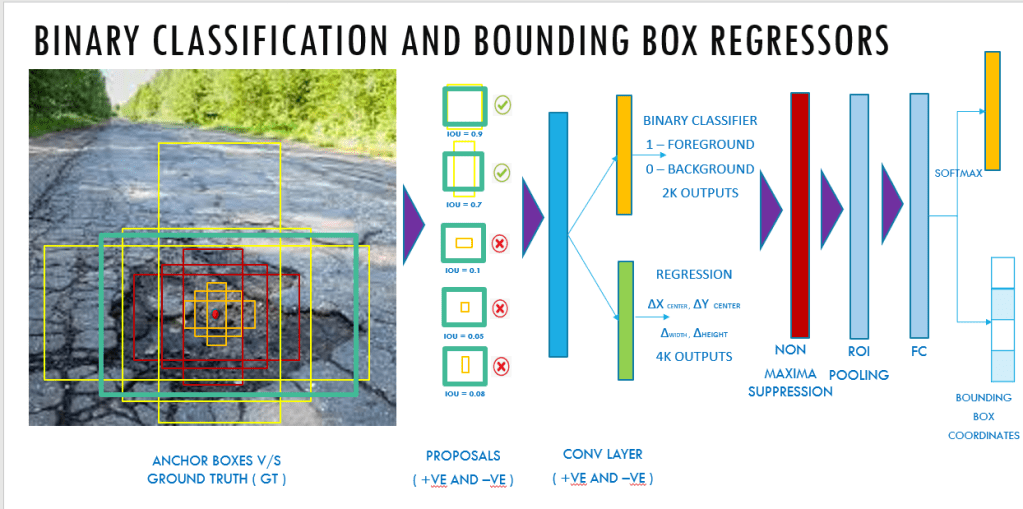
The binary classifier classifies the proposals as foreground ( containing an object) and background ( no object) and the regressor outputs the delta or adjustments that needs to be made to the reference anchor box, to make it similar to the ground truth bounding boxes. After these two steps in the RPN layer, the proposals are sorted based on the probability score as to whether it is foreground and background and then it undergoes Non maxima suppression to reduce the overlapping bounding boxes.

The reduced number of bounding boxes are then propogated to an ROI pooling layer which reduces the dimensions and then goes through the fully connected layers to the final softmax layers and the regressor layers. The softmax layer detects what type of object it is ( whether it is a pothole or vegetation or sign board etc) and the regressor layer gives the adjusted bounding boxes to that object.

One of the biggest advantages Faster RCNN has achieved over the previous versions is that all the moving parts can be integrated as one single network along with considerable speed in its implementation. We will leave the implementation of Faster RCNN to the subsequent chapter, where you could implement it using Tensorflow object detection API.

Having got an overview of the RCNN family, let us get to the implementation of the RCNN network.

Implementation of pothole object detector using RCNN

Let us quickly get an overview of the steps involved in the implementation of the object detector using RCNN

Creation of data sets with both positive and negative images. For creation of the data sets, we will be using the image annotation details we created in post 2. We will be using the same csv file which we created in post 2.
Use transfer learning technique to build our classifier. The pre-trained model we will be using is the MobileNetV2
Fine tune the pre-trained model as the classifier and save the model
Perform selective search algorithm using opencv for generating regions of proposals
Classify the proposal regions using the fine tuned Image net model
Perform non maxima suppression on the proposal regions

Let us start by importing the packages we require for this implementation

import os
import glob
import pandas as pd
import io
import cv2
import h5py
import numpy as np

from tensorflow.keras.preprocessing.image import ImageDataGenerator
from tensorflow.keras.applications import MobileNetV2
from tensorflow.keras.layers import AveragePooling2D
from tensorflow.keras.layers import Dropout
from tensorflow.keras.layers import Flatten
from tensorflow.keras.layers import Dense
from tensorflow.keras.layers import Input
from tensorflow.keras.models import Model
from tensorflow.keras.optimizers import Adam
from tensorflow.keras.applications.mobilenet_v2 import preprocess_input
from tensorflow.keras.preprocessing.image import img_to_array
from tensorflow.keras.preprocessing.image import load_img
from tensorflow.keras.utils import to_categorical
from tensorflow.keras.models import load_model
from sklearn.preprocessing import LabelBinarizer
from sklearn.model_selection import train_test_split
from sklearn.metrics import classification_report
from sklearn.feature_extraction.image import extract_patches_2d
from imutils import paths
import matplotlib.pyplot as plt
import pickle
import imutils

Data Preprocessing

For data preprocessing we have to convert the data and labels into arrays for us to train our models. We have two classes of data i.e the positive class which pertains to the potholes and the negative class which are those images other than potholes. We have to preprocess both these images seperately.

Let us start the process with the positive class. We will be using the ‘csv’ file which we created in Post 2 for getting the required information on the positive classes. Let us read the csv files and create two empty lists to store the data and labels.

# Reading the csv file
pothole_df = pd.read_csv('pothole_df.csv')

Let us explore the head of the positive class information data frame

pothole_df.head()

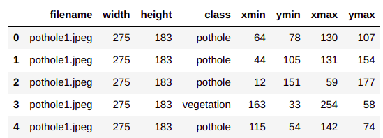
Each row of the data frame contains information on the file name of our image along with the localisation information of the pothole. We will be using these information to extract the region of interest ( roi ) from the image. Let us now get to creating the roi’s from this information. To start off we will create two empty lists to store the roi features and the labels.

# Empty lists to store data and labels
data = []
labels = []

Next we will create a function to extract the region of interest(roi’s) from the positive class. This class is similar to the one which we created in the previous post.

Region of interest Extractor for positive and negative classes

# Functions to extract the bounding boxes and preprocess the image
def roiExtractor(row,path):
    img = cv2.imread(path + row['filename'])    
    # Get the bounding box elements
    bb = [int(row['xmin']),int(row['ymin']),int(row['xmax']),int(row['ymax'])]
    # Crop the image
    roi = img[bb[1]:bb[3], bb[0]:bb[2]]
    # Reshape the image
    roi = cv2.resize(roi,(224,224),interpolation=cv2.INTER_CUBIC)    
    # Convert the image to an array
    roi = img_to_array(roi)
    # Preprocess the image
    roi = preprocess_input(roi)    
    return roi

The inputs to the function are each row of the csv file and the path to the folder where the images are placed. We first read the image in line 39.The image is read by concatenating the path to the images folder and the filename listed in the csv file. Once the image is read, the bounding box information for the image is extracted in line 41 and then the image is cropped to get only the positive classes in line 43. The images are then resized to a standard size of (224,224 )in line 45. We resize it to a standard dimension as that is the dimension required for the Mobilenet network. In lines 47-49, the images are converted to arrays and then preprocessed. The preprocess_input() method in line 49 normalises the pixel values so that it is between 0-1.

We will process the images based on the function we just created. We iterate through each row of the csv file ( line 54) and then extract only those rows where the class is ‘pothole’ ( line 55). We get the roi using the roiExtractor function ( line 56) and then append the roi to the list we created (data) ( line 58). The labels for the positive class are also appended to labels ( line 59) .

# This is the path where the images are placed. Change this path to the location you have defined
path = 'data/'
# Looping through the excel sheet rows
for idx, row in pothole_df.iterrows():    
    if row['class'] == 'pothole':
        roi = roiExtractor(row,path)
        # Append the data and labels for the positive class
        data.append(roi)
        labels.append(int(1))

print(len(data))
print(data[0].shape)

I have 31 roi’s of the positive class with a shape of (224,224,3).

Having processed the positive examples, let us now extract the negative examples. As seen in the previous post the negative classes are general images of roads without potholes.

# Listing all the negative examples
path = 'data/Annotated'
roadFiles = glob.glob(path + '/*.jpeg')
print(len(roadFiles))

I have selected 21 negative examples. You are free to get as many of these examples as possible. Only point which should be ensured is that there should be a good balance between the positive and negative class. We will now process the negative class images

# Looping through the images of negative class
for row in roadFiles:
    # Read the image
    img = cv2.imread(row)
    # Extract patches
    patches = extract_patches_2d(img,(128,128),max_patches=2)
    # For each patch do the augmentation
    for patch in patches:        
        # Reshape the image
        roi = cv2.resize(patch,(224,224),interpolation=cv2.INTER_CUBIC)
        #print(roi.shape)
        # Convert the image to an array
        roi = img_to_array(roi)
        # Preprocess the image
        roi = preprocess_input(roi)
        #print(roi.shape)
        # Append the data into the data folder and labels folder
        data.append(roi)
        labels.append(int(0))

For the negative classes, we iterate through each of the images and then read them in line 69. We then extract two patches each of size (128,128) from the image in line 71. Each patch is then resized to the standard size and the converted to array and preprocessed in lines 75-80. Finally the patches are appended to data and labels are appended as ‘0’.

Let us now take a count of the total examples we have

print(len(data))

We now have 73 examples which comprises of 31 positive classes and 42 ( 21 x 2 patches each ) negative classes.

Preparing the train and test sets

We will now convert the data and labels into arrays and then perform one hot encoding to the labels for preperation of our train and test sets.

# convert the data and labels to NumPy arrays
data = np.array(data, dtype="float32")
labels = np.array(labels)
print(data.shape)
print(labels.shape)

# perform one-hot encoding on the labels
lb = LabelBinarizer()
# Fit transform the labels array
labels = lb.fit_transform(labels)
# Convert this to categorical 
labels = to_categorical(labels)
print(labels.shape)
labels

After one hot encoding the labels array is transformed into a shape (73,2), where the second dimension is the class label. The first class is our negative class [0] and the second one is the positive class [1].

Finally let us create our train and test sets using a 85:15 split. We are taking a higher proportion of train set since we have very less training examples.

# Partition data to train and test set with 85 : 15 split
(trainX, testX, trainY, testY) = train_test_split(data, labels,test_size=0.15, stratify=labels, random_state=42)
print("training data shape :",trainX.shape)
print("testing data shape :",testX.shape)
print("training labels shape :",trainY.shape)
print("testing labels shape :",testY.shape)

Now that we have finished the data processing its time to start our training process

Training a MobilenetV2 model using transfer learning : Warming up phase

We will be building our object detector model using transfer learning process. To build our transfer learned model for pothole detection we will be using MobileNetV2 as our base network. We will remove the top layer and then build our custom layer to cater to our use case. Let us see how we build our network.

# Create the base network by removing the top of the MobileNetV2 model
baseNetwork = MobileNetV2(weights="imagenet", include_top=False,input_tensor=Input(shape=(224, 224, 3)))
# Create a custom head network on top of the basenetwork to cater to two classes.
topNetwork = baseNetwork.output
topNetwork = AveragePooling2D(pool_size=(5, 5))(topNetwork)
topNetwork = Flatten(name="flatten")(topNetwork)
topNetwork = Dense(128, activation="relu")(topNetwork)
topNetwork = Dropout(0.5)(topNetwork)
topNetwork = Dense(2, activation="softmax")(topNetwork)
# Place our custom top layer on top of the base layer. We will only train the base layer.
model = Model(inputs=baseNetwork.input, outputs=topNetwork)
# Freeze the base network so that they are not updated during the training process
for layer in baseNetwork.layers:
    layer.trainable = False

We load the base network in line 106. The base network is the MobileNetV2 and we exclude the top layer by specifying the parameter , include_top=False. We also specify the shape of the input layer.

Its now time to specify our custom network. We build our custom network on top of the output of the base network as shown in line 108. From lines 109-112, we build the different layers of our custom layer starting with the AveragePooling layer and the final Dense layer. In line 113 we define the final Softmax layer for our 2 classes. We then define the model using the Model() class with the inputs as the baseNetwork input and the output as the custom network we have defined in line 115.

In line 117, we specify which layers needs to be trained. Here we are specifying that the base network layers need not be trained. This is because the base network is already pre-trained and our custom layer is the one which is not trained. By specifying that only our custom layer be trained ( or alternatively the base network need not be trained), we are optimising the custom layer. This process can be called the warming up process for the custom layer. Once the custom layer is warmed up after some iterations, we can even specify that some layers of the base network too can be trained. We will perform all these steps.

First let us train our custom layer. We start off the process by defining our training parameters like learning rate, number of epochs and the batch size.

# Initialise the learning rate, epochs and batch size
LR = 1e-4
epoc = 5
bs = 16

You might be surprise that the epochs we have selecte is only 5. This is because since the base network is pre-trained we dont have to train the custom layer for many epochs. Besides we are only warming up the custom layer.

Next let us define the data generator along with the augmentation layer.

# Create a image generator with data augmentation
aug = ImageDataGenerator(rotation_range=40,zoom_range=0.25,width_shift_range=0.2,height_shift_range=0.2,shear_range=0.30,
 horizontal_flip=True,fill_mode="nearest")

In the previous post we implemented manual data augmentation methods. Keras has a great method to do image augmentation during training using the ImageDataGenerator(). It lets us do all the augmentation we did manually in the previous post.

We have now defined most of the moving parts required for training. Lets now define the optimiser and then compile the model and then fit the model with the data set.

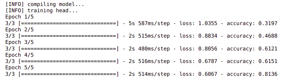
# Compile the model
print("[INFO] compiling model...")
opt = Adam(lr=LR)
model.compile(loss="binary_crossentropy", optimizer=opt,metrics=["accuracy"])
# Training the customer head network
print("[INFO] training the model...")
history = model.fit(aug.flow(trainX, trainY, batch_size=bs),steps_per_epoch=len(trainX) // bs,validation_data=(testX, testY),
 validation_steps=len(testX) // bs,epochs=epoc)

Training some layers of the base network

We have done the warm up of the custom head we placed over the base network. Now let us also train some of the layers of the network along with the head. Let us first print out all the layers of the base network to determine the layers we want to train along with our head.

for (i,layer) in enumerate(baseNetwork.layers):
    print(" [INFO] {}\t{}".format(i,layer.__class__.__name__))

In line 134, we iterate through each of the layers of the base network and the print the name of the layer.

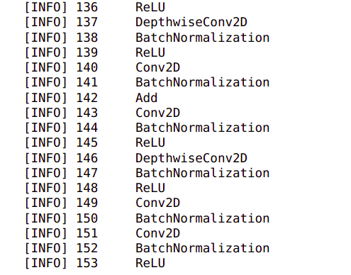
We can see that there are 153 layers in the base network. Let us train from layer 140 onwards and freeze all the layers above 140.

for layer in baseNetwork.layers[140:]:
    layer.trainable = True

# Compile the model
print("[INFO] Compiling the model again...")
opt = Adam(lr=LR)
model.compile(loss="binary_crossentropy", optimizer=opt,metrics=["accuracy"])
# Training the customer head network
print("[INFO] Fine tuning the model along with some layers of base network...")
history = model.fit(aug.flow(trainX, trainY, batch_size=bs),steps_per_epoch=len(trainX) // bs,validation_data=(testX, testY),
 validation_steps=len(testX) // bs,epochs=epoc)

With the new training we can see that the accuracy has jumped to 98% from the initial 80%. Let us predict on test set and then print the classification report.

For generating the classification report let us convert the label names into a string as shown below

# Converting the target names as string for classification report
target_names = list(map(str,lb.classes_))

Let us now print the classification report and see how well our model is performing on the test set

# make predictions on the test set
print("[INFO] Generating inference...")
predictions = model.predict(testX, batch_size=bs)
# For each prediction we need to find the index with maximum probability 
predIdxs = np.argmax(predictions, axis=1)
# Print the classification report
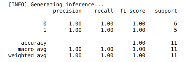
print(classification_report(testY.argmax(axis=1), predIdxs,target_names=target_names))

We get the predictions which are in the form of probabilities for each class in line 151. We then extract the id of the class which has the maximum probability using the np.argmax method in line 153. Finally we generate the classification report in line 155. We can see that we have a near perfect classification report as shown below.

Let us also visualise our training accuracy and loss and then save the figure.

# plot the training loss and accuracy
N = epoc
plt.style.use("ggplot")
plt.figure()
plt.plot(np.arange(0, N), history.history["loss"], label="train_loss")
plt.plot(np.arange(0, N), history.history["accuracy"], label="train_acc")
plt.title("Training Loss and Accuracy")
plt.xlabel("Epoch #")
plt.ylabel("Loss/Accuracy")
plt.legend(loc="lower left")
plt.savefig("plot.png")
plt.show()

Let us finally save our model and the label binarizer so that we can use it later in our inference process

MODEL_PATH = "output/pothole_detector_RCNN.h5"
ENCODER_PATH = "output/label_encoder_RCNN.pickle"
# serialize the model to disk
print("[INFO] saving pothole detector model...")
model.save(MODEL_PATH, save_format="h5")
# serialize the label encoder to disk
print("[INFO] saving label encoder...")
f = open(ENCODER_PATH, "wb")
f.write(pickle.dumps(lb))
f.close()

We have completed the training cycle and have saved the model. Let us now implement the inference cycle.

Inference run for pothole detection

In the inference cycle, we will use the model we just built to localise and predict potholes in test images. Let us first load the model and the label encoder which we saved.

MODEL_PATH = "output/pothole_detector_RCNN.h5"
ENCODER_PATH = "output/label_encoder_RCNN.pickle"
print("[INFO] loading model and label binarizer...")
model = load_model(MODEL_PATH)
lb = pickle.loads(open(ENCODER_PATH, "rb").read())

We have downloaded some test files. Lets visualise some of them here

# Please change the path where your files are placed
testpath = 'data/test'
testFiles = glob.glob(testpath + '/*.jpeg')
testFiles

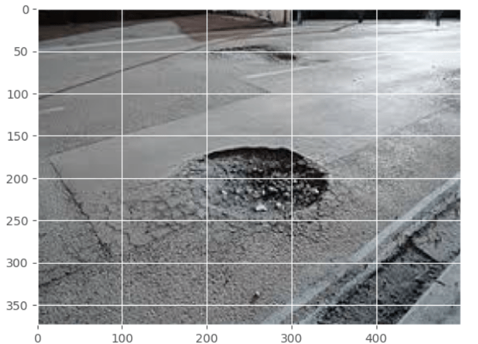
Lets plot one of the images

# load the input image from disk
image = cv2.imread(testFiles[2])
#Resize the image and plot the image
image = imutils.resize(image, width=500)
plt.imshow(image,aspect='equal')
plt.show()

We will use Opencv to generate the bounding boxes proposals for the image. Detailed below are the specific steps for the selective search implementation using Opencv to generate the bounding boxes. The set of proposals would be contained in the variable rects

# Implementing selective search to generate bounding box proposals
print("[INFO] running selective search and generating bounding boxes...")
ss = cv2.ximgproc.segmentation.createSelectiveSearchSegmentation()
ss.setBaseImage(image)
ss.switchToSelectiveSearchFast()
rects = ss.process()

Let us look how many proposals the selective search algorithm has generated

len(rects)

For this specific image as you can see the selective search algorithm has generated 920 proposals. As you know these are regions where there is high probability to find an object. As you might have noticed this specific algorithm is pretty slow in identifying all the bounding boxes.

Next let us extract the region of interest from the image using the bounding boxes we obtained from the selective search algorithm. Let us explore the code

# Initialise lists to store the region of interest from the image and its bounding boxes
proposals = []
boxes = []
max_proposals = 100
# Iterate over the bounding box coordinates to extract region of interest from image
for (x, y, w, h) in rects[:max_proposals]:    
    # Crop region of interest from the image
	roi = image[y:y + h, x:x + w]
    # Convert to RGB format as CV2 has output in BGR format
	roi = cv2.cvtColor(roi, cv2.COLOR_BGR2RGB)
    # Resize image to our standar size
	roi = cv2.resize(roi, (224,224),
		interpolation=cv2.INTER_CUBIC)
	# Preprocess the image
	roi = img_to_array(roi)
	roi = preprocess_input(roi)
	# Update the proposal and bounding boxes
	proposals.append(roi)
	boxes.append((x, y, x + w, y + h))

In lines 200-201, we initialise two lists for storing the roi’s and their bounding box co-oridinates. In line 202, we also define the max number of proposals we want. This step is to improve the speed of computation by eliminating processing of too many proposals. This is a parameter you can vary and I would encourage you to try out different values for this parameter.

Next we iterate through each of the bounding boxes we want, to extract the region of interest and their bounding boxes as detailed in lines 205-215. The various processes we implement are to crop the images, covert the images to RGB format, resize to the desired size and the final normalization of the pixel values. Finally the roi and bounding boxes are updated in lines 217-218 to the lists we created earlier.

Its now time to classify the regions of proposal using the model we fine tuned. Before classification we have to convert the lists to a numpy array. Let us implement these processes.

# Convert proposals and bouding boxes to NumPy arrays
proposals = np.array(proposals, dtype="float32")
boxes = np.array(boxes, dtype="int32")
print("[INFO] proposal shape: {}".format(proposals.shape))
# Classify the proposals based on the fine tuned model
print("[INFO] classifying proposals...")
proba = model.predict(proposals)

Next we will extract those roi’s which are classified as ‘potholes’ from the overall predictions.

# Find the predicted labels 
labels = lb.classes_[np.argmax(proba, axis=1)]
# Get the ids where the predictions are 'Potholes'
idxs = np.where(labels == 1)[0]
idxs

The model prediction gives us the probability of each class. We will find the predicted labels from the probability by taking the argmax of the predicted class probabilities as shown in line 227. Once we have the labels, we extract the indexes of the pothole class in line 229, which in our case is 1.

Next using the indexes we will extract the bounding boxes and probability of the ‘pothole’ class

# Using the indexes, extract the bounding boxes and prediction probabilities of 'pothole' class
boxes = boxes[idxs]
proba = proba[idxs][:, 1]

Next we will apply another filter and take only those bounding boxes which has a probability greater than a threshold value.

print(len(boxes))
# Filter the bounding boxes using a prediction probability threshold
pred_threshold = 0.995
# Select only those ids where the probability is greater than the threshold
idxs = np.where(proba >= pred_threshold)
boxes = boxes[idxs]
proba = proba[idxs]
print(len(boxes))

The threshold has been fixed in this case by experimenting with different values. This is another hyperparameter which needs to be arrived at observing the predictions you obtain for your specific set of images. We can see that before filtering we had 97 bounding boxes which has got reduced to 22 after the filtering. These filtered bounding boxes will be used to localise potholes on the image. Let us visualise the filtered bounding boxes on the image.

# Clone the original image for visualisation and inserting text
clone = image.copy()
# Iterate through the bounding boxes and associated probabilities
for (box, prob) in zip(boxes, proba):
    # Draw the bounding box, label, and probability on the image
    (startX, startY, endX, endY) = box
    cv2.rectangle(clone, (startX, startY), (endX, endY),(0, 255, 0), 2)
    # Initialising the cordinate for writing the text
    y = startY - 10 if startY - 10 > 10 else startY + 10
    # Getting the text to be attached on top of the box
    text= "Pothole: {:.2f}%".format(prob * 100)
    # Visualise the text on the image
    cv2.putText(clone, text, (startX, y),cv2.FONT_HERSHEY_SIMPLEX, 0.25, (0, 255, 0), 1)
# Visualise the bounding boxes on the image
plt.imshow(clone,aspect='equal')
plt.show()

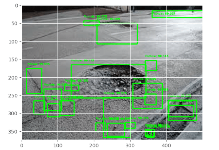
We clone the image in line 243 and then iterate through the boxes in lines 245 – 254. When we iterate through each box and grab the co-ordinates in line 247 and first draw the rectangle over the image with those co-ordinates in line 248. In the subsequent lines we print the class name and also the probability of the class on top of the bounding box. Finally we visualise the image with the bounding boxes and the text in lines 256-257.

As we can see we have the bounding boxes over the potholes and also regions around them also. However we can see that we have multiple overlapping boxes which ultimately needs to be reduced. So our next task is to apply non maxima suppression to reduce the number of bounding boxes.

Non Maxima Suppression

We will use the same method we used in the previous post for the non maxima suppression. Let us get the function for non maxima suppression. For explanation on this function please refer the previous post

def maxOverlap(boxes):
    '''
    boxes : This is the cordinates of the boxes which have the object
    returns : A list of boxes which do not have much overlap
    '''
    # Convert the bounding boxes into an array
    boxes = np.array(boxes)
    # Initialise a box to pick the ids of the selected boxes and include the largest box
    selected = []
    # Continue the loop till the number of ids remaining in the box is greater than 1
    while len(boxes) > 1:
        # First calculate the area of the bounding boxes 
        x1 = boxes[:, 0]
        y1 = boxes[:, 1]
        x2 = boxes[:, 2]
        y2 = boxes[:, 3]
        area = (x2 - x1) * (y2 - y1)
        # Sort the bounding boxes based on its area    
        ids = np.argsort(area)
        #print('ids',ids)
        # Take the coordinates of the box with the largest area
        lx1 = boxes[ids[-1], 0]
        ly1 = boxes[ids[-1], 1]
        lx2 = boxes[ids[-1], 2]
        ly2 = boxes[ids[-1], 3]
        # Include the largest box into the selected list
        selected.append(boxes[ids[-1]].tolist())
        # Initialise a list for getting those ids that needs to be removed.
        remove = []
        remove.append(ids[-1])
        # We loop through each of the other boxes and find the overlap of the boxes with the largest box
        for id in ids[:-1]:
            #print('id',id)
            # The maximum of the starting x cordinate is where the overlap along width starts
            ox1 = np.maximum(lx1, boxes[id,0])
            # The maximum of the starting y cordinate is where the overlap along height starts
            oy1 = np.maximum(ly1, boxes[id,1])
            # The minimum of the ending x cordinate is where the overlap along width ends
            ox2 = np.minimum(lx2, boxes[id,2])
            # The minimum of the ending y cordinate is where the overlap along height ends
            oy2 = np.minimum(ly2, boxes[id,3])
            # Find area of the overlapping coordinates
            oa = (ox2 - ox1) * (oy2 - oy1)
            # Find the ratio of overlapping area of the smaller box with respect to its original area
            olRatio = oa/area[id]            
            # If the overlap is greater than threshold include the id in the remove list
            if olRatio > 0.40:
                remove.append(id)                
        # Remove those ids from the original boxes
        boxes = np.delete(boxes, remove,axis = 0)
        # Break the while loop if nothing to remove
        if len(remove) == 0:
            break
    # Append the remaining boxes to the selected
    for i in range(len(boxes)):
        selected.append(boxes[i].tolist())
    return np.array(selected)

Let us now apply the non maxima suppression function and eliminate the overlapping boxes.

# Applying non maxima suppression
selected = maxOverlap(boxes)
len(selected)

We can see that by applying non maxima suppression we have reduced the number of boxes from 22 to around 3. Let us now visualise the images with the selected list of bounding boxes after non maxima suppression.

clone = image.copy()
plt.imshow(image,aspect='equal')
for (startX, startY, endX, endY) in selected:
    cv2.rectangle(clone, (startX, startY), (endX, endY), (0, 255, 0), 2)       

plt.imshow(clone,aspect='equal')
plt.show()

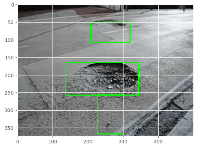
We can see that the number of bounding boxes have considerably reduced and have localised well to the two potholes.

With this we have come to the end of object detection using RCNN. Let us quickly recap what we have achieved in this post.

We preprocessed the positive and negative classes of images and then built our train and test sets
Fine tuned the MobileNet model to cater to our use case and made it our classifier.
Built the inference pipeline using the fine tuned classifier
Applied non maxima suppression to get the bounding boxes over the potholes.

We have come a long way and are now adept at implementing an advanced model like RCNN. However there are still variations to this model which we could try. One of the variations we can try is to implement a RCNN for multiple classes. So lets say we predict potholes and also road signs with the same network. Implementing a multiclass RCNN would adopt the same processes with a little variation during the model architecture and training. We will build a multiclass RCNN framework in a future post.

What Next ?

Having seen an advanced method like RCNN, we will go to another advanced method in the next post, which is Yolo. Yolo is a more faster method than RCNN and will enable us to use the road detection process in video files. We will be covering pothole detection using Yolo in the next post and then use it to detect potholes on videos in the subsequent post. Watch this space for more.

To be notified of the next post please subscribe to this blog post .You can also subscribe to our Youtube channel for all the videos related to this series.

You can also access the code base for this series from the following git hub link

Do you want to Climb the Machine Learning Knowledge Pyramid ?

Knowledge acquisition is such a liberating experience. The more you invest in your knowledge enhacement, the more empowered you become. The best way to acquire knowledge is by practical application or learn by doing. If you are inspired by the prospect of being empowerd by practical knowledge in Machine learning, subscribe to our Youtube channel

I would also recommend two books I have co-authored. The first one is specialised in d eep learning with practical hands on exercises and interactive video and audio aids for learning