“True knowledge come with deep understanding of a topic and its inner working”
Albert Einsteen
This is the fourth part of the series where we continue on our quest to understand the innerworking of a LSTM model. Deep understanding of the model is a step towards acquiring comprehensive knowledge on our machine translation application. This series comprises of 8 posts.
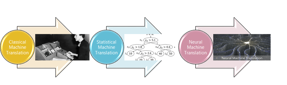
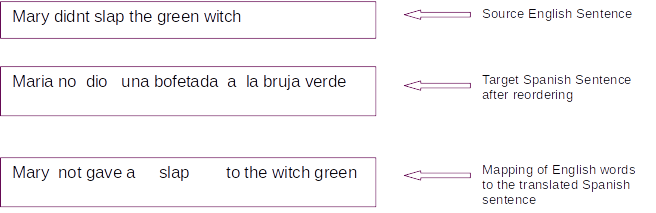
- Understand the landscape of solutions available for machine translation
- Explore sequence to sequence model architecture for machine translation.
- Deep dive into the LSTM model with worked out numerical example.
- Understand the back propagation algorithm for a LSTM model worked out with a numerical example.( This post)
- Build a prototype of the machine translation model using a Google colab / Jupyter notebook.
- Build the production grade code for the training module using Python scripts.
- Building the Machine Translation application -From Prototype to Production : Inference process
- Build the machine translation application using Flask and understand the process to deploy the application on Heroku
In the previous 3 posts we understood the solution landscape for machine translation ,explored different architecture choices for sequence to sequence models and did a deep dive into the forward propagation algorithm. Having understood the forward propagation its now time to explore the back propagation of the LSTM model
Back Propagation Through Time
We already know that Recurrent networks have a time component and we saw the calculations of different components during the forward propogation phase. We saw in the previous post that we traversed one time step at a time to get the expected outputs.

The backpropagation operation works in the reverse order and traverses one time step at a time in the reverse order to get the gradients of all he parameters. This process is called back propagation through time.
The initiation step of the back propagation is the error term .As you know the dynamics of optimization entails calculating the error between the predicted output and ground truth, propagating the gradient of the error to the layers thereby updating the parameters of the model. The work horse of back propagation is partial differentiation,using the chain rule. Let us see that in action.
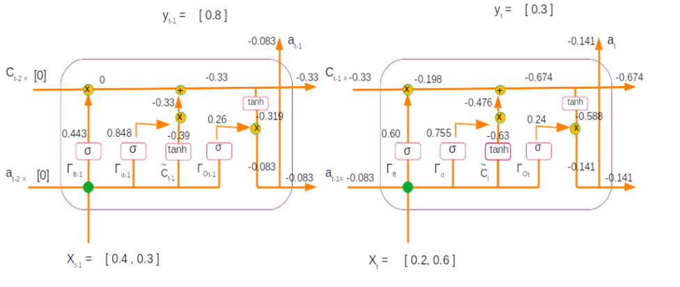
Backpropagation calculation @ time step 2
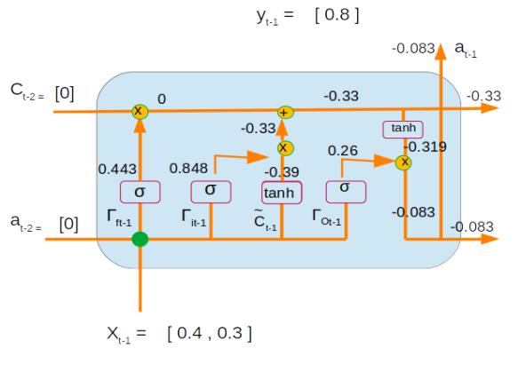
We start with the output from our last layer which as calculated in the forward propagation stage is ( refer the figure above)
a t = -0.141
The label for this time step is
Yt = 0.3
In this toy example we will take a simple loss function , a squared loss. The error would be derived as the average of squared difference between the last time step and the ground truth (label).
Error = ( at – yt )2/2
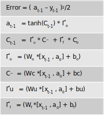
Before we start the back propagation it would be a good idea to write down all the equations in the order in which we will be taking the derivative.
Error = ( at – yt )2/2at = tanh( Ct ) * ҐoCt = Ґu * C~ + Ґf * Ct-1Ґo = sigmoid(Wo *[xt , at-1] + bo)C~ = tanh(Wc *[xt , at-1] + bc)Ґu = sigmoid(Wu *[xt , at-1] + bu)Ґf = sigmoid(Wf *[xt , at-1] + bf)
We mentioned earlier that the dynamics of backpropogation is the propogation of the gradients . But why is getting the gradients important and what information does it carry ? Let us answer these questions.
A gradient represents unit rate of change i.e the rate at which parameters have to change to get a desired reduction in error. The error which we get is dependent on how close to reality our initial assumptions of weights were. If our initial assumption of weights were far off from reality, the error also would be large and viceversa. Now our aim is to adjust our initial weights so that the error is reduced. This adjustment is done through the back propagation algorithm. To make the adjustment we need to know the quantum of adjustment and also the direction( i.e whether we have to add or subtract the adjustments from initially assumed weights). To derive the quantum and direction we use partial differentiation. You would have learned in school that partial differentiation gives you the rate of change of a variable with respect to another. In this case we need to know the rate at which the error would change when we make adjustments to our assumed parameters like weights and bias terms.
Our goal is to get the rate of change of error with respect to the weights and the biases. However if you look at our first equation
Error = ( at – yt )2/2
we can see that it dosent have any weights in it. We only have the variable at . But we know from our forward propagation equations that at is derived by different operations involving weights and biases. Let us traverse downwards from the error term and trace out different trails to the weights and biases.
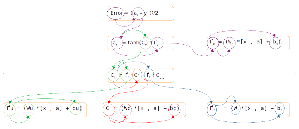
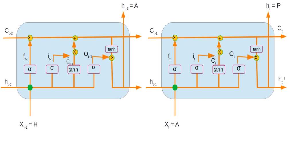
The above figure represents different trails ( purple,green,red and blue ) to reach the weights and biases from the error term. Let us first traverse the purple coloured trail.
The purple coloured trail is to calculate the gradients associated with the output gate. When we say gradients it entails finding the rate of change of the error term with respect to the weights and biases associated with the output gate, which in mathematical form is represented as ∂E/∂Wo. If we look down the purple trail we can see that Wo appears in the equation at the tail end of the trail. This is where we apply the chain rule of differentiation. Chain rule of differentiation helps us to differentiate the error with respect to the connecting links till we get to the terms which we want, like weights and biases. This operation can be represented using the following equation.

The green coloured trail is a longer one. Please note that the initial part of the green coloured trail, where the differentiation with respect to error term is involved ( ∂E/∂a ), is the same as the purple trail. From the second box onwards a distinct green trail takes shape and continues till the box with the update weight (Wu). The equation for this can be represented as follows
∂E/∂Wu = ∂E/∂a * ∂a/∂Ct * ∂Ct/ ∂Γu * ∂Γu/∂Wu
The other trails are similar. We will traverse through each of these trails using the numerical values we got after the forward propagation stage in the last post.
Gradients of Equation 1 : Error = ( at – yt )2/2
The first step in backpropagation is to take the derivative of the error with respect to at
dat = ∂E/∂at = ∂/∂at[ (at -y)2/2]
= 2 * (at-y)/ 2
= at-y
Let us substitute the values
| Derivative 2.1.1. | Numerical Eqn | Value |
| dat = at– y | = -0.141 – 0.3 | -0.441 |
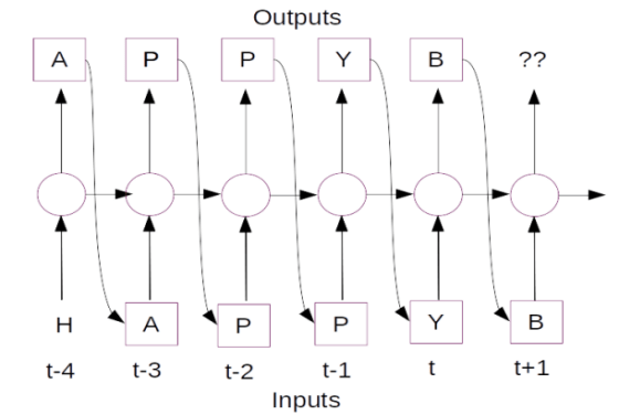
If you are thinking that thats all for this term then you are in for a surprise. In the case of a sequence model like LSTM there would be an error term associated with each time step and also an error term which back propagates from the previous time step. The error term for certain time step would be the sum total of both these errors. Let me explain this pictorially.
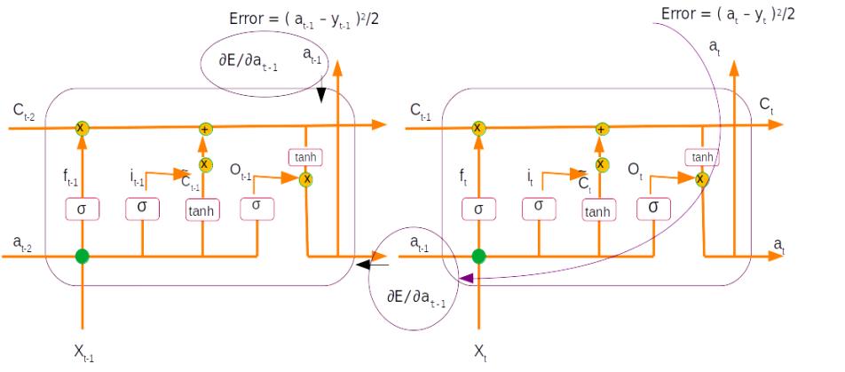
Let us assume that we are taking the derivative of the error with respect to the output from the first time step (∂E/∂at-1), which is represented in the above figure as the time step on the left. Now if you notice the same output term at-1 is also propogated to the second time step during the forward propagation stage. So when we take the derivative there is a gradient of this output term which is with respect to the error from the second time step. This gets propogated through all the equations within the second time step using the chain rule as represented by the purple arrow. This gradient has to be added to the gradient derived from the first time step to get the final gradient for that output term.
However in the case of the top example since we are taking the gradient of the second time step and there are no further time step, this term which gets propogated from the previous time step would be 0. So ideally the equation for the derivative for the second output should be written as follows
| Derivative – 1.1 | Numerical Eqn | Value |
| da = at – y + 0 | = -0.141 – 0.3 + 0 | -0.441 |
In this equation ‘0’ corresponds to the gradient from the third time step, which in this case dosent exist.
Gradients of Equation 2 : [at = tanh( Ct ) * Ґo ]
Having found the gradient for the first equation which had the error term, the next step is to find the gradient of the output term at and its component terms Ct and Ґo.

Let us first differentiate it with respect to Ct. The equations for this step are as follows
∂E/∂Ct = ∂E/∂at * ∂at/∂Ct
= da * ∂at/∂Ct
In this equation we have already found the value of the first term which is ∂E/∂at in the first step. Next we have to find the partial derivative of the second term ∂at/∂Ct
∂at/∂Ct = Γo * ∂/∂Ct [ tanh(Ct)]
= Γo * [1 - tanh2(Ct)]
Please note => ∂/∂x [ tanh(x)]= 1 – tanh2(x)
So the complete derivation for ∂E/∂Ct is
∂E/∂Ct = da * Γo * [1 - tanh2(Ct)]
So the above is the derivation of the partial derivative with respect to state 2. Well not quite. There is one more term to be added to this where state 2 will appear. Let me demonstrate that. Let us assume that we had 3 time steps as shown in the table below
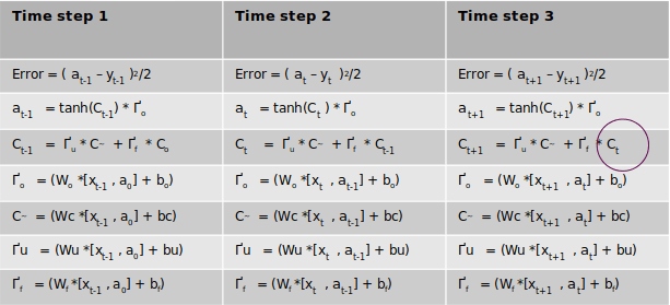
We can see that the term Ctappears in the 3rd time step as circled in the table. When we take the derivative of error of time step 2 with respect to Ct we will have to take the derivative from the third time step also. However in our case since the third step doesn’t exist that term will be ‘0’ as of now. However when we take the derivative of the first time step we will have to consider the corresponding term from the second time step. We will come to that when we take the derivative of the first time step. For the time being it is ‘0’ for us now as there is no third time step.
| Derivative – 2.2.1 | Numerical Eqn | Value |
| dCt = da * Ґo * (1 – tanh2(Ct ) + 0 | = -0.441 * 0.24* (1-tanh2(-0.674 ) = -0.441 * 0.24* ( 1 – (-0.59 * -0.59)) | -0.069 |
Let us now take the gradient with the second term of equation 2 which is Ґo. The complete equation for this term is as follows
∂E/Γo = ∂E/∂at * ∂at/∂Γo
= da * ∂at/∂Γo
The above equation is very similar to the earlier derivation. However there are some nuances with the derivation of the term with Γo . If you remember this term is a sigmoid gate with the following equation.
Γo = sigmoid(Wo *[xt , at-1] + bo)
= sigmoid(u)
Where u = Wo *[xt , at-1] + bo
When we take the derivative of the output term with respect to Γo (∂at/∂Γo ), this should be with respect to the terms inside the sigmoid function ( u). So ∂at/∂Γo would actually mean ∂at/∂u . So the entire equation can be rewritten as
at = tanh(Ct) * sigmoid(u) where Γo = sigmoid(u).
Therefore ∂at/∂Γo = tanh(Ct) * Γo *( 1 - Γo )
Please note if y = sigmoid(x) , ∂y/∂x = y(1-y)
The complete equation for the term ∂E/Γo =
da * tanh(Ct) * Γo *( 1 - Γo )
Substituting the numerical terms we get
| Derivative – 2.2.2 | Numerical Eqn | Value |
| d Ґ0 = da *tanh(Ct)* Ґo *(1 – Ґo) | = -0.441 * tanh(-0.674) * 0.24 *(1-0.24) | 0.047 |
Gradients of Equation 3 : [ Ct = Ґu * C~ + Ґf * Ct-1 ]
Let us now find the gradients with respect to the third equation
This equation has 4 terms, Ґu, C~ , Ґf and Ct-1 , for which we have to calculate the gradients. Let us start from the first term Ґu whose equation is the following
∂E/Γu = ∂E/∂at * ∂at/∂Ct * ∂Ct/ ∂Γu
However the first two terms of the above equation, ∂E/∂at * ∂at/∂Ct were already calculated in derivation 2.1, which can be represented as dCt . The above equation can be re-written as
∂E/Γu = dCt * ∂Ct/ ∂Γu
From the new equation we are left with the second part of the equation which is ∂Ct / ∂Γu ,which is the derivative of equation 3 with respect to Γu.
Ct = Ґu * C~ + Ґf * Ct-1.......... (3)
∂Ct/Γu = C~ * ∂/ ∂Γu [ Ґu ] + 0.........(3.1)
In equation 3 we can see that there are two components, one with the term Ґu in it and the other with Ґf in it. The partial derivative of the first term which is partial derivative with respect to Ґu is what is represented in the first half of equation 3.1. The partial derivative of second half which is the part with the gate Ґf will be 0 as there is no Ґu in it. Equation 3.1 represents the final form of the partial derivative.
Now similar to derivative 2.2 which we developed earlier, the partial derivative of the sigmoid gate ∂/ ∂Γu [ Ґu ] will be Γu * ( 1 - Γu ). The final form of equation 3.1 would be
∂Ct/Γu = C~ * Γu * ( 1 - Γu )
The solution for the gradient with respect to the update gate would be
∂E/Γu = dCt* C~ * Γu * ( 1 - Γu )
| Derivative 2.3.1 | Numerical Eqn | Value |
| d Ґu = dCt *C~* Ґu *(1 – Ґu) | = -0.069 * -0.63 * 0.755 *(1-0.755) | 0.0080 |
Next let us calculate the gradient with respect to the internal state C~ . The complete equation for this is as follows
∂E/C~ = ∂E/∂at * ∂at/∂Ct * ∂Ct/ ∂C~
= dCt * ∂Ct/ ∂C~
= dCt * ∂/ ∂C~ [ Ґu * C~]
= dCt * Ґu * ∂/ ∂C~ [ C~]
However we know that, C~ = tanh(Wc *[x , a] + bc) . Let us represent the terms within the tanh function as u .
C~ = tanh(u), where u = Wc *[x , a] + bc
Similar to the derivations we have done for the sigmoid gates, we take the derivatives with respect to the terms within the tanh() function which is ‘u’ . Therefore
∂/ ∂C~ [ C~] = 1-tanh2 (u)
= 1 - tanh2 (Wc *[x , a] + bc)
= 1 - (C~ )2
since, C~ = tanh(Wc *[x , a] + bc) and therefore
(C~ )2 = tanh2 (Wc *[x , a] + bc)
The final equation for this term would be
∂E/C~ = dCt * Ґu * 1 - (C~ )2
| Derivative 2.3.2 | Numerical Eqn | Value |
| dC~ = dCt* Ґu * (1 – (C~)2) | = -0.069 * 0.755 * (1-(-0.63)2) | -0.0314 |
The gradient with respect to the third term Ґf would be very similar to the derivation of the first term Ґu
∂E/Γf = ∂E/∂at * ∂at/∂Ct* ∂Ct/ ∂Γf
= dCt* Ct-1 * Γf * ( 1 - Γf )
| Derivative 2.3.3 | Numerical Eqn | Value |
| d Ґf = dCt* Ct-1* Ґf *(1 – Ґf) | = -0.069 * -0.33 * 0.60 *(1-0.60) | 0.0055 |
Finally we come to the gradient with respect to the fourth term Ct-1 ,the equation for which is as follows
∂E/Ct-1 = ∂E/∂at * ∂at/∂Ct* ∂Ct/ ∂Ct-1
= dCt* Γf
| Derivative 2.3.4 | Numerical Eqn | Value |
| dCt-1 = dCt *Ґf | = -0.069 * 0.60 | -0.0414 |
In this step we have got the gradient of cell state 1 which will come in handy when we find the gradients of time step 1.
Gradients of previous time step output (at-1)
In the previous step we calculated the gradients with respect to equation 3. Now it is time to find the gradients with respect to the output from time step 1 , at-1.
However one fact which we have to be cognizant is that at-1 is present in 4 different equations, 4,5,6 & 7. So we have to take derivative with respect to all these equations and then sum it up. The gradient of at-1 within equation 4 is represented as below
∂E/∂at-1 = ∂E/∂at * ∂at/∂Ct * ∂Ct/ ∂Γo * ∂Γo/∂at-1
However we have already found the gradient of the first three terms of the above equation, which is with respect to the terms within the sigmoid function i.e ‘u’ as dΓo in derivative 2.1. Therefore the above equation can be simplified as
∂E/∂at-1 = dΓo * ∂Γo/∂at-1
The term ∂Γo/∂at-1 in reality is ∂u/∂at-1 where u = Wo *[x , at-1] + bo, because when we took the derivative of Γo we took it with respect to all the terms within the sigmoid() function,which we called as ‘u’.
From the above equation the derivative will take the form
∂Γo/∂at-1 = ∂u/∂at-1 = Wo
The complete equation from the gradient is therefore
∂E/∂at-1 = dΓo * Wo
There are some nuances to be taken care in the above equation since there is a multiplication by Wo . When we looked at the equation for the forward pass we saw that to get the equation of the gates, we originally had two weights, one for the x term and the other for the ‘a’ term as below
Ґo = sigmoid(Wo*[x ] + Uo* [a] + bo)
This equation was simplified by concatenating both the weight parameters and the corresponding x & a vectors to a form given below.
Ґo = sigmoid(Wo *[x , a] + bo)
So in effect there is a part of the final weight parameter Wo which is applied to ‘x’ and another part which is applied to ‘a’. Our initial value of the weight parameter Wo was [-0.75 ,-0.95 , -0.34]. The first two values are the values corresponding to ‘x’ as it is of dimension 2 and the last value ( -0.34) is what is applicable for ‘a’. So in our final equation for the gradient of at-1, ∂E/∂at-1 = dΓo * Wo , we will multiply dΓo only with -0.34.
Similar to the above equation we have to take the derivative of at-1for all other equations 5,6 and 7 which will take the form
Equation 5 = > ∂E/∂at-1 = dC~* Wc
Equation 6= > ∂E/∂at-1 = dΓu* Wu
Equation 7 = > ∂E/∂at-1 = dΓf* Wf
The final equation of will be the sum total of all these components
| Derivative 2.4.1 | Numerical Eqn | Value |
| dat-1 = Wo * dҐo + Wc * dC~ + Wu * dҐu + Wf * dҐf | = [(-0.34 * 0.047) + (-0.13 * -0.0314) + (1.31 * 0.0080) + (-0.13*0.0055) ] | -0.00213 |
Now that we have calculated the gradients of all the components for time step 2, let us proceed with the calculations for time step 1
Back Propagation @ time step 1.
All the equations and derivations for time step 1 is similar to time step 2. Let us calculate the gradients of all the equations as we did with time step 1
Gradients of Equation 1 : Error term
Gradient with respect to error term of the current time step
| Derivative 1.1.1 | Numerical Eqn | Value |
| dat-1 = at-1 – yt-1 | = -0.083 – 0.8 | -0.883 |
However we know that dat-1 = Gradient with respect current layer + Gradient from next time step, as shown in the figure below

Gradient propagated from the 2nd layer is the derivative of at-1which was derived as the last step of the previous time step ( Derivative 2.4.1)
Total Gradient
| Derivative 1.1.1 | Numerical Eqn | Value |
| dat-1 = Gradient from this layer + Gradient from previous layer | = -0.883 + -0.00213 | -0.88513 |
Gradients of Equation 2
Next we have to find the gradients of equation 2 with respect to the cell state, Ct-1and Ґo.When deriving gradient of cell state state we discussed that the cell state of the current layer appears in the next layer also, which will have to be considered. So the total derivative would be
| Derivative 1.2.1 | Formulae |
| dCt-1 = dCt-1 in current time step + dCt-1 from next time step | dCt-1 = da * Ґo * (1 – tanh2(Ct-1 ) + dCt-1 *Ґf ( Derivative 3.4) |
| Derivative 1.2.1 | Numerical Eqn | Value |
| dCt-1 = da * Ґo * (1 – tanh2(Ct-1 ) + dCt-1in next layer | = -0.88513 * 0.26 * (1-tanh2(-0.33 ) + (-0.0414) = -0.88513* 0.26 * ( 1 – (-0.319 * -0.319)) – 0.0414 | -0.25 |
Next is the gradient with respect to Ґo .
| Derivative 1.2.2 | Numerical Eqn | Value |
| d Ґ0 = da *tanh(Ct-1)* Ґo *(1 – Ґo) | = -0.88513 * tanh(-0.33) * 0.26 *(1-0.26) | 0.054 |
Gradients of Equation 3
- Derivative with respect to Ґu
| Derivative 1.3.1 | Numerical Eqn | Value |
| d Ґu = dCt-1 *C~* Ґu *(1 – Ґu) | = -0.25 * -0.39 * 0.848 *(1-0.848) | 0.013 |
- Derivative with respect to C~
| Derivative 1.3.2 | Numerical Eqn | Value |
| dC~ = dCt-1 * Ґu * (1 – (C~)2) | = -0.25 * 0.848 * (1-(-0.39)2) | -0.18 |
- Derivative with respect to Ґf
| Derivative 1.3.3 | Numerical Eqn | Value |
| d Ґf = dCt-1 *C0* Ґf *(1 – Ґf) | = -0.25 * 0 * 0.443 *(1-0.443) | 0 |
- Derivative with respect to initial cell state C<0>
| Derivative 1.3.4 | Numerical Eqn | Value |
| dC0 = dCt-1 *Ґf | = -0.25 * 0.443 | -0.11 |
Gradients of initial output (a0)
Similar to the previous time step this has 4 components pertaining to equations 4,5,6 & 7
| Derivative 1.4.1 | Numerical Eqn | Value |
| da0 = Wo * dҐo + Wc * dC~ + Wu * dҐu + Wf * dҐf | = [(-0.34 * 0.054) + (-0.13 * -0.18) + (1.31 * 0.013) + (-0.13*0) ] | 0.022 |
Now that we have completed the gradients for both time steps let us tabularize the results of all the gradients we have got so far
| Eqn | Gradients | Values |
| 2.1.1 | dat = at – yt + 0 | 0.441 |
| 2.2.1 | dCt = dat * Ґo * (1 – tanh2(Ct ) + 0 | -0.069 |
| 2.2.2 | d Ґ0 = dat * tanh(Ct )* Ґo *(1 – Ґo) | 0.047 |
| 2.3.1 | d Ґu = dCt * C~ * Ґu *(1 – Ґu) | 0.0080 |
| 2.3.2 | dC~ = dCt * Ґu * (1 – (C~)2) | -0.0314 |
| 2.3.3 | d Ґf = dCt * Ct-1 * Ґf *(1 – Ґf) | 0.0055 |
| 2.3.4 | dCt-1 = dCt * Ґf | -0.0414 |
| 2.4.1 | dat-1 = Wo * dҐo + Wc * dC~ + Wu * dҐu + Wf * dҐf | -0.00213 |
| 1.1.1 | dat-1 = at-1 – yt-1 + eq (2.4.1) | -0.88513 |
| 1.2.1 | dCt-1 = dat-1 * Ґo * (1 – tanh2(Ct-1 ) + eq 2.3.4 | -0.25 |
| 1.2.2 | d Ґ0 = dat-1 * tanh(Ct-1 )* Ґo *(1 – Ґo) | 0.054 |
| 1.3.1 | d Ґu = dCt-1* C~ * Ґu *(1 – Ґu) | 0.013 |
| 1.3.2 | dC~ = dCt-1* Ґu * (1 – (C~)2) | -0.18 |
| 1.3.3 | d Ґf = dCt-1 * C0 * Ґf *(1 – Ґf) | 0 |
| 1.3.4 | dC0 = dCt-1 * Ґf | -0.11 |
| 1.4.1 | da0 = Wo * dҐo + Wc * dC~ + Wu * dҐu + Wf * dҐf | 0.022 |
Gradients with respect to weights
The next important derivative which we have to derive is with respect to the weights. We have to remember that the weights of an LSTM is shared across all the time steps. So the derivative of the weight will be the sum total of the derivatives from each individual time step. Let us first define the equation for the derivative of one of the weights, Wu.
The relevant equation for this is the following

The first three terms of the gradient is equal to dҐu which was already derived through equations 2.3.1 and 1.3.1 in the table above. Also remember dҐu is the gradient with respect to the terms inside the sigmoid function ( i.e Wu *[xt , at-1] + bu) . Therefore the derivative of the last term, ∂Γu/∂Wu would be
∂Γu/∂Wu = [xt , at-1]
The complete equation for the gradient with respect to the weight Wu would be
∂E/∂Wu = dҐu * [xt , at-1]
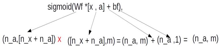
The important thing to note in the above equation is the dimensions of each of the terms. The first term, dҐu, is a scalar of dimension (1,1) , however the second term is a vector of dimension (1 ,3) . The resultant gradient would be another vector of dimension (1,3) as the scalar value will be multiplied with all the terms of the vector. We will come to that shortly. However for now let us find the gradients of all other weights.The derivation for other weights are similar to the one we saw. The equations for the gradients with respect to all weights for time step 1 are as follows
| Derivative | Equation |
| dWf | = dҐf * [xt , at-1] |
| dWo | = dҐo * [xt , at-1] |
| dWc | = dC~ * [ xt , at-1] |
| dWu | = dҐu * [xt , at-1] |
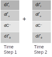
The total weight derivative would be sum of weight derivatives of all the time steps.
dW = dW1 + dW2
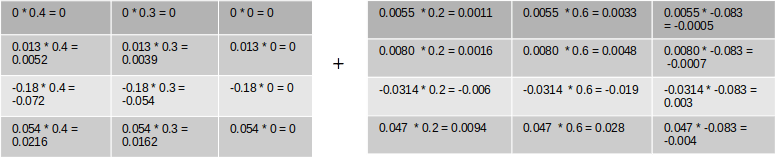
As discussed above to find the total gradient it would be convenient and more efficient to stack all these equations in a matrix form and then multiply it with the input terms and then adding them across the different time steps. This operation can be represented as below

Let us substitue the numberical values and calculate the gradients for the weights

The matrix multiplication will have the following values
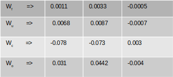
The final gradients for all the weights are the following
Gradients with respect to biases
The next task is to get the gradients of the bias . The derivation of the gradients for bias is similar to that of the weights. The equation for the bias terms would be as follows

Similar to what we have done for the weights, the first three terms of the gradient is equal to dҐu . The derivative of the fourth term which are the terms inside the sigmoid function ( i.e Wu *[xt , at-1] + bu) will be
∂Γu/∂bu = 1
The complete equation for the gradient with respect to the weight Wu would be
∂E/∂bu = dҐu * 1
The final gradient of the bias term would be the sum of the gradients of the first time step and the second. As we have seen in case of the weights, the matrix form would be as follows
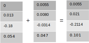
The final gradients for the bias terms are
Weights and bias updates
Calculating the gradients using back propagation is not an end by itself. After the gradients are calculated, they are used to update the initial weights and biases .
The equation is as follows
Wnew = Wold - α * Gradients
Here α is a constant which is the learning rate. Let us assume it to be 0.01
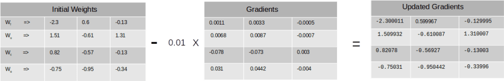
The new weights would be as follows
Similarly the updated bias would be

As you would have learned, these updated weights and bias terms would take the place of the initial weights and biases in the next forward pass and then the back progagation again kicks in to calculate the new set of gradients which will be applied on the updated weights and gradients to get the new set of parameters. This process will continue till the pre-defined epochs.
Error terms when softmax is used
The toy example which we saw just now has a squared error term, which was used for backpropagation. The adoption of such an example was only to demonstrate the concepts with a simple numerical example. However in the problem which we are dealing with or for that matter many of the problems which we will deal with will have a softmax layer as its final layer and thereafter cross entropy as its error function. How would the backpropogation derivation differ when we have a different error term than what we have just done in the toy example ? The major change would be in terms of how the error term is generated and how the error is propogated till the output term at. After this step the flow will be the same as what we we have seen earlier.
Let us quickly see an example for a softmax layer and a cross entropy error term. To demonstrate this we will have to revisit the forward pass from the point we generate the output from each layer.
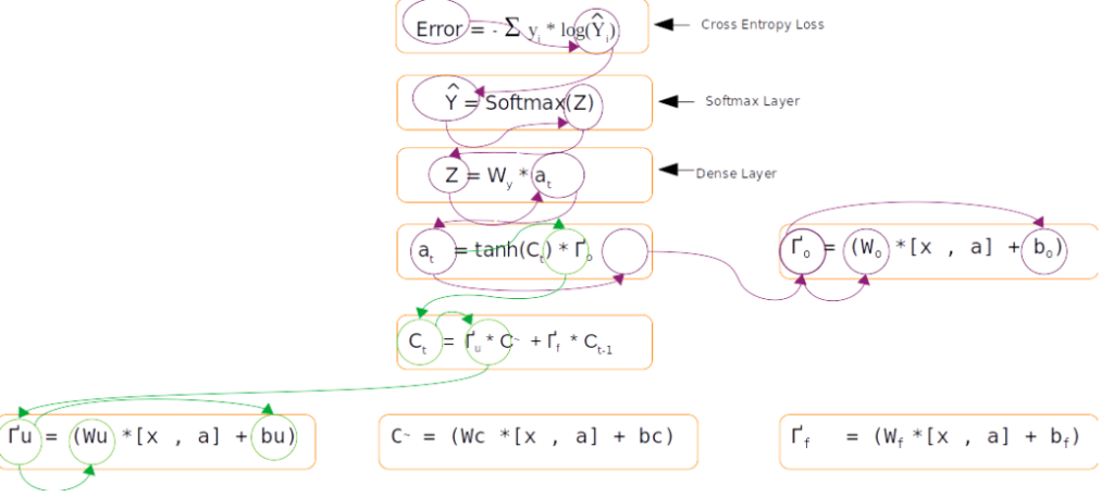
The above figure is a representation of the equations for the forward pass and backward pass of an LSTM. Let us look at each of those steps
Dense Layer
We know that the output layer at from a LSTM will be a vector with dimension equal to number of units of the LSTM. However for the application which we are trying to build the output we require is the most probable word in the target vocabulary. For example if we are translating from German to English, given a German sentence, for each time step we need to predict a corresponding English word. The prediction from the final layer would be in the form of a probability distribution over all the words in the English vocabulary we have in our corpus.
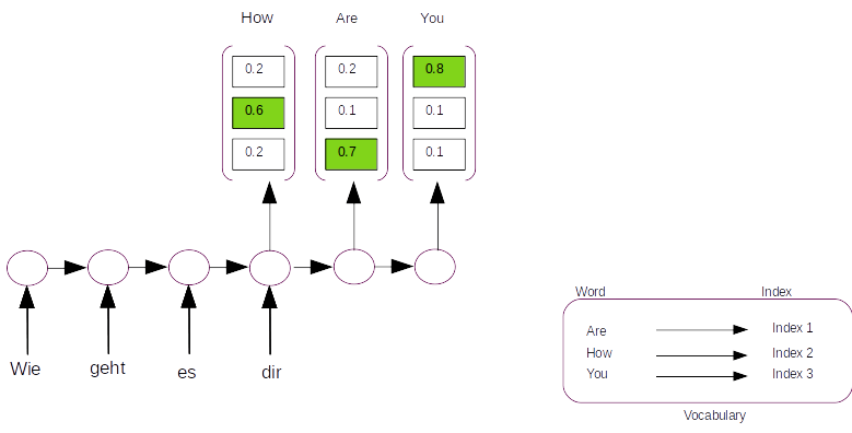
Let us look at the above representation to understand this better. We have an input German sentence 'Wie geht es dir' which translates to 'How are you'. For simiplicity let us assume that there are only 3 words in the target vocabulary ( English vocabulary). Now the predictions will have to be a probability distribution over the three words over the target vocabulary and the index which has the highest probability will be the prediction. In the prediction we see that the first time step has the maximum probability ( 0.6) on the second index which corresponds to the word ‘How’ in the vocabulary. The second and third time steps have maximum probability on the first and third indexes respectively giving us the predicted string as ‘How are you’. ( Please note that in the figure above the index of the probability is from bottom to top, which means the bottom most box corresponds to index 1 and top most to index 3)
Coming back to our equation, the output layer at is only a vector and not a probability distribution. To get a probability distribution we need to have a dense layer and a final softmax layer. Let us understand the dynamics of how the conversion from the output layer to the probability distribution happens.
The first stage is the dense layer where the output layer vector is converted to a vector with the same dimension as of the vocabulary. This is achieved by the multiplication of the output vector with the weights of the dense layer. The weight matrix will have the dimension [ length of vocabulary , num of units in output layer]. So if there are 3 words in the vocabulary and one unit in the output layer then weight matrix will be of dimension [ 3, 1], ie it has 3 rows and one column. Another way of seeing this dimension is each row of the weight matrix corresponds to each word in the vocabulary. The dense layer would be derived by the dot product of weight matrix with the output layer
Z = Wy * at
The dimensions of the resultant vector will be as follows
[3,1] * [1,1] => [3,1]
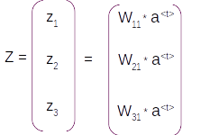
The resultant vector Z after the dense layer operation will have 3 rows and 1 column as shown below.
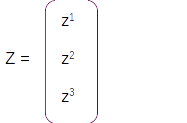
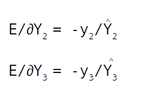
This vector is still not a probability distribution. To convert it to a probability distribution we take the softmax of this dense layer and the resultant vector will be a probability distribution with the same dimension.
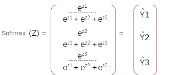
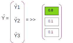
The resultant probability distribution will be called as Y^ which will have three components ( equal to the dimension of the vocabulary), each component will be the probability of the corresponding word in the vocabulary
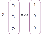
Having seen the forward pass let us look at how the back propogation works. Let us start with the error term which in this case will be cross entropy loss as this is a classification problem. The cross entropy loss will have the form

In this equation the term y is the true label in one hot encoded form. So if the first index ( y1) is the true label for this example the label vector in one hot encoded format will be
Now let us get into the motions of backpropogation. We need to back propogate till at after which the backpropogation equation will be the same as what we derived in the toy example. The complete back propogation equation till at according to the chain rule will be

Let us look at the derivations term by term
Back propogation derivation for first term
The first equation ∂E/∂Y^ is a differentiation with respect to a vector as Y^ ,having three components, Y1 , Y2 and Y3 . A differentiation with a vector is called a Jacobian which will again be a vector of the same dimension as Y.
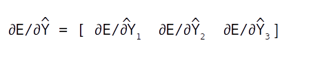
Let us look at deriving each of these terms within the vector
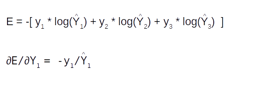
Please note ∂/∂y(Logy) = 1/y
Similarly we get
So the Jacobian of ∂E/∂Y^ will be

Suppose the first label (y1) is the true label. Then the one hot encoded form which is [ 1 0 0 ] will make the above Jacobian

Back propogation derivation for second term
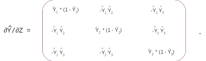
Let us do the derivation for the second term ∂Y^/∂Z . This term is a little more interesting as both the Y and Z are vectors. The differentiation will result a Jacobian matrix of the form

Let us look at the first row and get the derivatives first. To recap let us look at the equations involved in the derivatives
Let us take the derivative of the first term ∂Y1^/∂Z1 . This term will be the derivative of the first element in the matrix
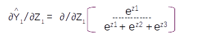
Taking the derivation based on the division rule of differentiation we get

Please note ∂/∂y(ey) = ey
Taking the common terms in the numerator and denominator and re-arranging the equation we get

Dividing through inside the bracket we get
Which can be simplified as

Since

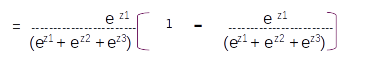
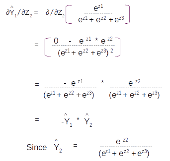
Let us take the derivative of the second term ∂Y1^/∂Z2 . This term will be the derivative of the first element in the matrix with respect to Z2
With these two derivations we can get all the values of the Jacobian. The final form of the Jacobian would be as follows
Well that was a long derivation. Now to get on to the third term.
Back propogation derivation for third term
Let us do the derivation for the last term ∂Z/ ∂at . We know from the dense layer we have
Z = Wy * at
So in vector form this will be
So when we take the derivation we get another Jacobian vector of the form

So thats all in this derivation. Now let us tie everything together to get the derivative with respect to the output term using the chain rule
Gradient with respect to the output term
We earlier saw that the equation of the gradient as
Let us substitute with the derivations which we already found out

The dot product of the first two terms will get you

The dot product of the above term with the last vector will give you the result you want

This is the derivation till ∂E/∂at . The rest of the derivation down from here to various components inside the LSTM layer will be the same as we have seen earlier in the toy example.
In terms of dimensions let us convince ourselves that we get the dimension equal to the dimension of ∂at
[1 , 3 ] * [3, 3] * [3, 1] ==> [1,1]
Wrapping up
That takes us to the end of the “Looking inside the hood” sessions for our model. In the two sessions we saw the forward propagation part of the LSTM cell and also derived the backward propagation part of the LSTM using toy examples. These examples are aimed at giving you an intuitive sense of what is going on inside the cells. Having seen the mathematical details, let us now get into real action. In the next post we will build our prototype using python on a Jupyter notebook. We will be implementing the encoder decoder architecture using LSTM. Having equipped with the nuances of the encoder decoder architecture and also the inner working of the LSTM you would be in a better position to appreciate the models which we will be using to build our Machine translation application.
Go to article 5 of this series : Building the prototype using Jupyter notebook
Do you want to Climb the Machine Learning Knowledge Pyramid ?
Knowledge acquisition is such a liberating experience. The more you invest in your knowledge enhacement, the more empowered you become. The best way to acquire knowledge is by practical application or learn by doing. If you are inspired by the prospect of being empowerd by practical knowledge in Machine learning, I would recommend two books I have co-authored. The first one is specialised in deep learning with practical hands on exercises and interactive video and audio aids for learning

This book is accessible using the following links
The Deep Learning Workshop on Amazon
The Deep Learning Workshop on Packt
The second book equips you with practical machine learning skill sets. The pedagogy is through practical interactive exercises and activities.

This book can be accessed using the following links
The Data Science Workshop on Amazon
The Data Science Workshop on Packt
Enjoy your learning experience and be empowered !!!!


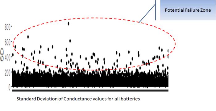


 The above is a plot depicting standard deviation of conductance for all batteries. Now what might be of interest to us is the red zone which we can call the “Potential failure Zone”. The potential failure zone consists of those batteries whose conductance values show high standard deviation. Batteries with failing health are likely to exhibit large fall in conductance and as a corollary their values will also show higher standard deviation. This implies that the samples of batteries which have higher probability of failure will in all likelihood be from this failure zone. However to ascertain this hypothesis we will have to dig deep into batteries in the failure zone and look for patterns which might differentiate them from normal batteries. Another objective to dig deep is also to elicit clues from the underlying patterns on what features to include in the predictive model. We will discuss more on the feature extraction when we discuss about feature engineering. Now let us come back to our discussion on digging deep into the failure zone and ferreting out significant patterns. It has to be noted that in addition to the samples in the failure zone we will also have to observe patterns from the normal zone to help separate wheat from the chaff . Intuitions derived by observing different patterns would become vital during feature engineering stage.
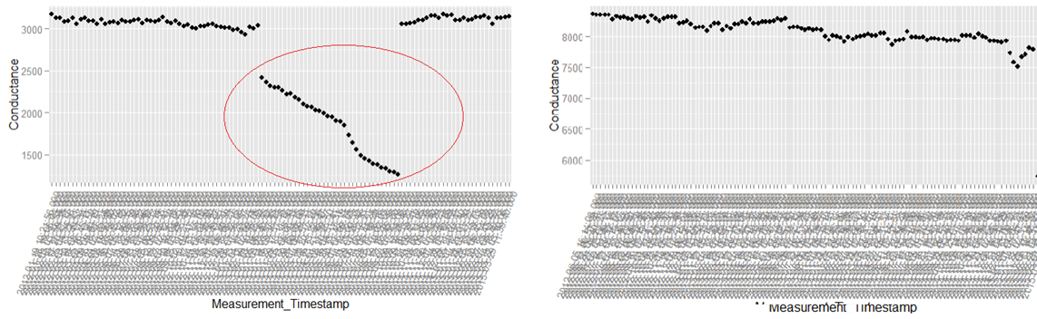
 .
.