

This is the sixth part of the series where we continue on our pursuit to build a machine translation application. In this post we embark on a transformation process where in we transform our prototype into a production grade code.
This series comprises of 8 posts.
- Understand the landscape of solutions available for machine translation
- Explore sequence to sequence model architecture for machine translation.
- Deep dive into the LSTM model with worked out numerical example.
- Understand the back propagation algorithm for a LSTM model worked out with a numerical example.
- Build a prototype of the machine translation model using a Google colab / Jupyter notebook.
- Build the production grade code for the training module using Python scripts.( This post)
- Building the Machine Translation application -From Prototype to Production : Inference process
- Build the machine translation application using Flask and understand the process to deploy the application on Heroku
In this section we will see how we can take the prototype which we built in the last article into a production ready code. In the prototype building phase we were developing our code on a Jupyter/Colab notebook. However if we have to build an application and deploy it, notebooks would not be very effective. We have to convert the code we built on the notebook into production grade code using python scripts. We will be progressively building the scripts using a process, I call, as the factory model. Let us see what a factory model is.
Factory Model
A Factory model is a modularized process of generating business outcomes using machine learning models. There are some distinct phases in the process which includes
- Ingestion/Extraction process : Process of getting data from source systems/locations
- Transformation process : Transformation process entails transforming raw data ingested from multiple sources into a form fit for the desired business outcome
- Preprocessing process: This process involves basic level of cleaning of the transformed data.
- Feature engineering process : Feature engineering is the process of converting the preprocessed data into features which are required for model training.
- Training process : This is the phase where the models are built from the featurized data.
- Inference process : The models which were built during the training phase is then utilized to generate the desired business outcomes during the inference process.
- Deployment process : The results of the inference process will have to be consumed by some process. The consumer of the inferences could be a BI report or a web service or an ERP application or any downstream applications. There is a whole set of process which is involved in enabling the down stream systems to consume the results of the inference process. All these steps are called the deployment process.
Needless to say all these processes are supported by an infrastructure layer which is also called the data engineering layer. This layer looks at the most efficient and effective way of running all these processes through modularization and parallelization.

All these processes have to be designed seamlessly to get the business outcomes in the most effective and efficient way. To take an analogy its like running a factory where raw materials gets converted into a finished product and thereby gets consumed by the end customers. In our case, the raw material is the data, the product is the model generated from the training phase and the consumers are any business process which uses the outcomes generated from the model.
Let us now see how we can execute the factory model to generate the business outcomes.
Project Structure
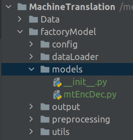
Before we dive deep into the scripts, let us look at our project structure.
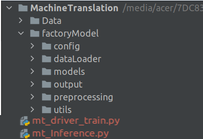
Our root folder is the Machine Translation folder which contains two sub folders Data and factoryModel. The Data subfolder contains the raw data. The factoryModel folder contains different subfolders containing scripts for our processes. We will be looking at each of these scripts in detail in the subsequent sections. Finally we have two driver files mt_driver_train.py which is the driver file for the training process and mt_Inference.py which is the driver file for the inference process.
Let us first dive into the training phase scripts.
Training Phase
The first part of the factory model is the training phase which comprises of all the processes till the creation of the model. We will start off by building the supporting files and folders before we get into the driver file. We will first start with the configuration file.
Configuration file
When we were working with the notebook files, we were at a liberty to change the pararmeters we wanted to vary, say for example the path to the input file or some hyperparameters like the number of dimensions of the embedding vector, on the notebook itself. However when an application is in production we would not have the luxury to change the parameters and hyperparameters directly in the code base. To get over this problem we use the configuration files. We consolidate all the parameters and hyperparameters of the model on to the configuration file. All processes will pick the parameters from the configuration file for further processing.
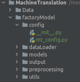
The configuration file will be inside the config folder. Let us now build the configuration file.
Open a word editor like notepad++ or any other editor of your choice and open a new file and name it mt_config.py. Let us start adding the below code in this file.
'''
This is the configuration file for storing all the application parameters
'''

import os
from os import path


# This is the base path to the Machine Translation folder
BASE_PATH = '/media/acer/7DC832E057A5BDB1/JMJTL/Tomslabs/BayesianQuest/MT/MachineTranslation'
# Define the path where data is stored
DATA_PATH = path.sep.join([BASE_PATH,'Data/deu.txt'])
Lines 5 and 6, we import the necessary library packages.
Line 10, we define the base path for the application. You need to change this path based on your specific path to the application. Once the base path is set, the rest of the paths will be derived out from it. In Line 12, we define the path to the raw data set folder. Note that we just join the name of the data folder and the raw text file with the base path to get the data path. We will be using the data path to read in the raw data.
In the config folder there will be another file named __init__.py . This is a special file which tells Python to treat the config folder as part of the package. This file inside this folder will be an empty file with no code in it
Loading Data
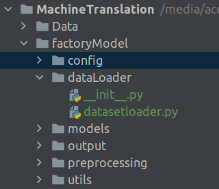
The next helper files we will build are those for loading raw files and preprocessing. The code we use for these purposes are the same code which we used for building the prototype. This file will reside in the dataLoader folder
In your text editor open a new file and name it as datasetloader.py and then add the below code into it
'''
Factory Model for Machine translation preprocessing.
This is the script for loading the data and preprocessing data
'''

import string
import re
from pickle import dump
from unicodedata import normalize
from numpy import array

# Creating the class to load data and then do the preprocessing as sequence of steps

class textLoader:
	def __init__(self , preprocessors = None):
		# This init method is to store the text preprocessing pipeline
		self.preprocessors = preprocessors
		# Initializing the preprocessors as an empty list of the preprocessors are None
		if self.preprocessors is None:
			self.preprocessors = []

	def loadDoc(self,filepath):
		# This is the function to read the file from the path provided
		# Open the file
		file = open(filepath,mode = 'rt',encoding = 'utf-8')
		# Reading the text
		text = file.read()
		#Once the file is read, applying the preprocessing steps one by one
		if self.preprocessors is not None:
			# Looping over all the preprocessing steps and applying them on the text data
			for p in self.preprocessors:
				text = p.preprocess(text)

		# Closing the file
		file.close()

		# Returning the text after all the preprocessing
		return text
Before addressing the code block line by line, let us get a big picture perspective of what we are trying to accomplish. When working with text you would have realised that different sources of raw text requires different preprocessing treatments. A preprocessing method which we have used for one circumstance may not be warranted in a different one. So in this code block we are building a template called textLoader, which reads in raw data and then applies different preprocessing steps like a pipeline as the situation warrants. Each of the individual preprocessing steps would be defined seperately. The textLoader class first reads in the data and then applies the selected preprocessing one after the other. Let us now dive into the details of the code.
Lines 6 to 10 imports all the necessary library packages for the process.
Line 14 we define the textLoader class. The constructor in line 15 takes the text preprocessor pipeline as the input. The prepreprocessors are given as lists. The default value is taken as None. The preprocessors provided in the constructor is initialized in line 17. Lines 19-20 initializes an empty list if the preprocessor argument is none. If you havent got a handle of why the preprocessors are defined this way, it is ok. This will be more clear when we define the actual preprocessors. Just hang on till then.
From line 22 we start the first function within this class. This function is to read the raw text and the apply the processing pipeline. Lines 25 – 27, where we open the text file and read the text is the same as what we defined during the prototype phase in the last post. We do a check to see if we have defined any preprocessor pipeline in line 29. If there are any pipeline defined those are applied on the text one by one in lines 31-32. The method .preprocess is specific to each of the preprocessor in the pipeline. This method would be clear once we take a look at each of the preprocessors. We finally close the raw file and the return the processed text in lines 35-38.
The __init__.py file inside this folder will contain the following line for importing the textLoader class from the datasetloader.py file for any calling script.
from .datasetloader import textLoader
Processing Data : Preprocessing pipeline construction
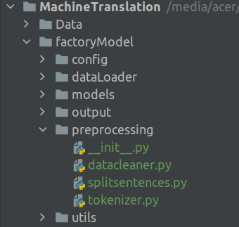
Next we will create the files for preprocessing the text. In the last section we saw how the raw data was loaded and then preprocessing pipeline was applied. In this section we look into the preprocessing pipeline. The folder structure will be as shown in the figure.
There would be three preprocessors classes for processing the raw data.
- SentenceSplit : Preprocessor to split raw text into pair of English and German sentences. This class is inside the file
splitsentences.py - cleanData : Preprocessor to apply cleaning steps like removing punctuations, removing whitespaces which is included in the
datacleaner.pyfile. - TrainMaker : Preprocessor to tokenize text and then finally prepare the train and validation sets contined in the
tokenizer.py file
Let us now dive into each of the preprocessors.
Open a new file and name it splitsentences.py. Add the following code to this file.
'''
Script for preprocessing of text for Machine Translation
This is the class for splitting the text into sentences
'''

import string
from numpy import array

class SentenceSplit:
	def __init__(self,nrecords):
		# Creating the constructor for splitting the sentences
		# nrecords is the parameter which defines how many records you want to take from the data set
		self.nrecords = nrecords

	# Creating the new function for splitting the text
	def preprocess(self,text):
		sen = text.strip().split('\n')
		sen = [i.split('\t') for i in sen]
		# Saving into an array
		sen = array(sen)
		# Return only the first two columns as the third column is metadata. Also select the number of rows required
		return sen[:self.nrecords,:2]
This is the first or our preprocessors. This preprocessor splits the raw text and finally outputs an array of English and German sentence pairs.
After we import the required packages in lines 6-7, we define the class in line 9. We pass a variable nrecords to the constructor to subset the raw text and select number of rows we want to include for training.
The preprocess function starts in line 16. This is the function which we were accessing in line 32 of the textLoader class which we discussed in the last section. The rest is the same code we have used in the prototype building phase which includes
- Splitting the text into sentences in line 17
- Splitting each sentece on tab spaces to get the German and English sentences ( line 18)
Finally we convert the processed sentences into an array and return only the first two columns of the array. Please note that the third column contains metadata of each line and therefore we exclude it from the returned array. We also subset the array based on the number of records we want.
Now that the first preprocessor is complete,let us now create the second preprocessor.
Open a new file and name it datacleaner.py and copy the below code.
'''
Script for preprocessing data for Machine Translation application
This is the class for removing the punctuations from sentences and also converting it to lower cases
'''

import string
from numpy import array
from unicodedata import normalize

class cleanData:
	def __init__(self):
		# Creating the constructor for removing punctuations and lowering the text
		pass

	# Creating the function for removing the punctuations and converting to lowercase
	def preprocess(self,lines):
		cleanArray = list()
		for docs in lines:
			cleanDocs = list()
			for line in docs:
				# Normalising unicode characters
				line = normalize('NFD', line).encode('ascii', 'ignore')
				line = line.decode('UTF-8')
				# Tokenize on white space
				line = line.split()
				# Removing punctuations from each token
				line = [word.translate(str.maketrans('', '', string.punctuation)) for word in line]
				# convert to lower case
				line = [word.lower() for word in line]
				# Remove tokens with numbers in them
				line = [word for word in line if word.isalpha()]
				# Store as string
				cleanDocs.append(' '.join(line))
			cleanArray.append(cleanDocs)
		return array(cleanArray)
This preprocessor is to clean the array of German and English sentences we received from the earlier preprocessor. The cleaning steps are the same as what we have seen in the previous post. Let us quickly dive in and understand the code block.
We start of by defining the cleanData class in line 10. The preprocess method starts in line 16 with the array from the previous preprocessing step as the input. We define two placeholder lists in line 17 and line 19. In line 20 we loop through each of the sentence pair of the array and the carry out the following cleaning operations
- Lines 22-23, normalise the text
- Line 25 : Split the text to remove the whitespaces
- Line 27 : Remove punctuations from each sentence
- Line 29: Convert the text to lower case
- Line 31: Remove numbers from text
Finally in line 33 all the tokens are joined together and appended into the cleanDocs list. In line 34 all the individual sentences are appended into the cleanArray list and converted into an array which is returned in line 35.
Let us now explore the third preprocessor.
Open a new file and name it tokenizer.py . This file is pretty long and therefore we will go over it function by function. Let us explore the file in detail
'''
This class has methods for tokenizing the text and preparing train and test sets
'''

import string
import numpy as np
from numpy import array
from tensorflow.keras.preprocessing.text import Tokenizer
from tensorflow.keras.preprocessing.sequence import pad_sequences
from sklearn.model_selection import train_test_split


class TrainMaker:
	def __init__(self):
		# Creating the constructor for creating the tokenizers
		pass

	# Creating an internal function for tokenizing the text
	def tokenMaker(self,text):
		tokenizer = Tokenizer()
		tokenizer.fit_on_texts(text)
		return tokenizer
We down load all the required packages in lines 5-10, after which we define the constructor in lines 13-16. There is nothing going on in the constructor so we can conveniently pass it over.
The first function starts on line 19. This is a function we are familiar with in the previous post. This function fits the tokenizer function on text. The first step is to instantiate the tokenizer object in line 20 and then fit the tokenizer object on the provided text in line 21. Finally the tokenizer object which is fit on the text is returned in line 22. This function will be used for creating the tokenizer dictionaries for both English and German text.
The next function which we will see is the sequenceMaker. In the previous post we saw how we convert text as sequence of integers. The sequenceMaker function is used for this task.
	# Creating an internal function for encoding and padding sequences

	def sequenceMaker(self,tokenizer,stdlen,text):
		# Encoding sequences as integers
		seq = tokenizer.texts_to_sequences(text)
		# Padding the sequences with respect standard length
		seq = pad_sequences(seq,maxlen=stdlen,padding = 'post')
		return seq
The inputs to the sequenceMaker function on line 26 are the tokenizer , the maximum length of a sequence and the raw text which needs to be converted to sequences. First the text is converted to sequences of integers in line 28. As the sequences have to be of standard legth, they are padded to the maximum length in line 30. The standard length integer sequences is then returned in line 31.
	# Creating another function to find the maximum length of the sequences
	def qntLength(self,lines):
		doc_len = []
		# Getting the length of all the language sentences
		[doc_len.append(len(line.split())) for line in lines]
		return np.quantile(doc_len, .975)
The next function we will define is the function to find the quantile length of the sentences. As seen from the previous post we made the standard length of the sequences equal to the 97.5 % quantile length of the respective text corpus. The function starts in line 34 where the complete text is given as input. We then create a placeholder in line 35. In line 37 we parse through each of the line and the find the total length of the sentence. The length of each sentence is stored in the placeholder list we created earlier. Finally in line 38, the 97.5 quantile of the length is returned to get the standard length.
	# Creating the function for creating tokenizers and also creating the train and test sets from the given text
	def preprocess(self,docArray):
		# Creating tokenizer forEnglish sentences
		eng_tokenizer = self.tokenMaker(docArray[:,0])
		# Finding the vocabulary size of the tokenizer
		eng_vocab_size = len(eng_tokenizer.word_index) + 1
		# Creating tokenizer for German sentences
		deu_tokenizer = self.tokenMaker(docArray[:,1])
		# Finding the vocabulary size of the tokenizer
		deu_vocab_size = len(deu_tokenizer.word_index) + 1
		# Finding the maximum length of English and German sequences
		eng_length = self.qntLength(docArray[:,0])
		ger_length = self.qntLength(docArray[:,1])
		# Splitting the train and test set
		train,test = train_test_split(docArray,test_size = 0.1,random_state = 123)
		# Calling the sequence maker function to create sequences of both train and test sets
		# Training data
		trainX = self.sequenceMaker(deu_tokenizer,int(ger_length),train[:,1])
		trainY = self.sequenceMaker(eng_tokenizer,int(eng_length),train[:,0])
		# Validation data
		testX = self.sequenceMaker(deu_tokenizer,int(ger_length),test[:,1])
		testY = self.sequenceMaker(eng_tokenizer,int(eng_length),test[:,0])
		return eng_tokenizer,eng_vocab_size,deu_tokenizer,deu_vocab_size,docArray,trainX,trainY,testX,testY,eng_length,ger_length
We tie all the earlier functions in the preprocess method starting in line 41. The input to this function is the English, German sentence pair as array. The various processes under this function are
- Line 43 : Tokenizing English sentences using the tokenizer function created in line 19
- Line 45 : We find the vocabulary size for the English corpus
- Lines 47-49 the above two processes are repeated for German corpus
- Lines 51-52 : The standard lengths of the English and German senetences are found out
- Line 54 : The array is split to train and test sets.
- Line 57 : The input sequences for the training set is created using the sequenceMaker() function. Please note that the German sentences are the input variable ( TrainX).
- Line 58 : The target sequence which is the English sequence is created in this step.
- Lines 60-61: The input and target sequences are created for the test set
All the variables and the train and test sets are returned in line 62
The __init__.py file inside this folder will contain the following lines
from .splitsentences import SentenceSplit
from .datacleaner import cleanData
from .tokenizer import TrainMaker
That takes us to the end of the preprocessing steps. Let us now start the model building process.
Model building Scripts
Open a new file and name it mtEncDec.py . Copy the following code into the file.
'''
This is the script and template for different models.
'''

from tensorflow.keras.models import Sequential
from tensorflow.keras.layers import LSTM
from tensorflow.keras.layers import Dense
from tensorflow.keras.layers import Embedding
from tensorflow.keras.layers import RepeatVector
from tensorflow.keras.layers import TimeDistributed

class ModelBuilding:
	@staticmethod
	def EncDecbuild(in_vocab,out_vocab, in_timesteps,out_timesteps,units):
		# Initializing the model with Sequential class
		model = Sequential()
		# Initiating the embedding layer for the text
		model.add(Embedding(in_vocab, units, input_length=in_timesteps, mask_zero=True))
		# Adding the first LSTM layer
		model.add(LSTM(units))
		# Using the RepeatVector to map the input sequence length to output sequence length
		model.add(RepeatVector(out_timesteps))
		# Adding the second layer of LSTM
		model.add(LSTM(units, return_sequences=True))
		# Adding the fully connected layer with a softmax layer for getting the probability
		model.add(TimeDistributed(Dense(out_vocab, activation='softmax')))
		# Compiling the model
		model.compile(optimizer='adam', loss='sparse_categorical_crossentropy')
		# Printing the summary of the model
		model.summary()
		return model
The model building scripts is straight forward. Here we implement the encoder decoder model we described extensively in the last post.
We start by importing all the necessary packages in lines 5-10. We then get to the meat of the model by defining the ModelBuilding class in line 12. The model we are using for our application is defined through a function EncDecbuild in line 14. The inputs to the function are the
in_vocab: This is the size of the German vocabularyout_vocab: This is the size of the Enblish vocabularyin_timesteps: The standard sequence length of the German sentencesout_timesteps: Standard sequence length of Enblish sentencesunits: Number of hidden units for the LSTM layers.
The progressive building of the model was covered extensively in the last post. Let us quickly run through the same here
- Line 16 we initialize the sequential class
- The next layer is the
Embeddinglayer defined in line 18. This layer converts the text to word embedding vectors. The inputs are the German vocabulary size, the dimension required for the word embeddings and the sequence length of the input sequences. In this example we have kept the dimension of the word embedding same as the number of units of LSTM. However this is a parameter which can be experimented with. - Line 20, we initialize our first LSTM unit.
- We then perform the Repeat vector operation in Line 22 so as to make the mapping between the encoder time steps and decoder time steps
- We add our second LSTM layer for the decoder part in Line 24.
- The next layer is the dense layer whose output size is equal to the English vocabulary size.(Line 26)
- Finally we compile the model using ‘adam’ optimizer and then summarise the model in lines 28-30
So far we explored the file ecosystem for our application. Next we will tie all these together in the driver program.
Driver Program
Open a new file and name it mt_driver_train.py and start adding the following code blocks.
'''
This is the driver file which controls the complete training process
'''

from factoryModel.config import mt_config as confFile
from factoryModel.preprocessing import SentenceSplit,cleanData,TrainMaker
from factoryModel.dataLoader import textLoader
from factoryModel.models import ModelBuilding
from tensorflow.keras.callbacks import ModelCheckpoint
from factoryModel.utils.helperFunctions import *

## Define the file path to input data set
filePath = confFile.DATA_PATH

print('[INFO] Starting the preprocessing phase')

## Load the raw file and process the data
ss = SentenceSplit(50000)
cd = cleanData()
tm = TrainMaker()
Let us first look at the library file importing part. In line 5 we import the configuration file which we defined earlier. Please note the folder structure we implemented for the application. The configuration file is imported from the config folder which is inside the folder named factoryModel. Similary in line 6 we import all three preprocessing classes from the preprocessing folder. In line 7 we import the textLoader class from the dataLoader folder and finally in line 8 we import the ModelBuilding class from the models folder.
The first task we will do is to get the path of the files which we defined in the configuration file. We get the path to the raw data in line 13.
Lines 18-20, we instantiate the preprocessor classes starting with the SentenceSplit, cleanData and finally the trainMaker classes. Please note that we pass a parameter to the SentenceSplit(50000) class to indicate that we want only 50000 rows of the raw data, for processing.
Having seen the three preprocessing classes, let us now see how these preprocessors are tied together in a pipeline to be applied sequentially on the raw text. This is achieved in next code block
# Initializing the data set loader class and then executing the processing methods
tL = textLoader(preprocessors = [ss,cd,tm])
# Load the raw data, preprocess it and create the train and test sets
eng_tokenizer,eng_vocab_size,deu_tokenizer,deu_vocab_size,text,trainX,trainY,testX,testY,eng_length,ger_length = tL.loadDoc(filePath)
Line 21 we instantiate the textLoader class. Please note that all the preprocessing classes are given sequentially in a list as the parameters to this class. This way we ensure that each of the preprocessors are implemented one after the other when we implement the textLoader class. Please take some time to review the class textLoader earlier in the post to understand the dynamics of the loading and preprocessing steps.
In Line 23 we implement the loadDoc function which takes the path of the data set as the input. There are lots of processes which goes on in this method.
- First loads the raw text using the file path provided.
- On the raw text which is loaded, the three preprocessors are implemented one after the other
- The last preprocessing step returns all the required data sets like the train and test sets along with the variables we require for modelling.
We now come to the end of the preprocessing step. Next we take the preprocessed data and train the model.
Training the model
We have already built all the necessary scripts required for training. We will tie all those pieces together in the training phase. Enter the following lines of code in our script
### Initiating the training phase #########
# Initialise the model
model = ModelBuilding.EncDecbuild(int(deu_vocab_size),int(eng_vocab_size),int(ger_length),int(eng_length),256)
# Define the checkpoints
checkpoint = ModelCheckpoint('model.h5',monitor = 'val_loss',verbose = 1, save_best_only = True,mode = 'min')
# Fit the model on the training data set
model.fit(trainX,trainY,epochs = 50,batch_size = 64,validation_data=(testX,testY),callbacks = [checkpoint],verbose = 2)
In line 34, we initialize the model object. Please note that when we built the script ModelBuilding was the name of the class and EncDecbuild was the method or function under the class. This is how we initialize the model object in line 34. The various parameter we give are the German and English vocabulary sizes, sequence lenghts of the German and English senteces and the number of units for LSTM ( which is what we adopt for the embedding size also). We define the checkpoint variables in line 36.
We start the model fitting in line 38. At the end of the training process the best model is saved in the path we have defined in the configuration file.
Saving the other files and variables

Once the training is done the model file is stored as a 'model.h5‘ file. However we need to save other files and variables as pickle files so that we utilise them during our inference process. We will create a script where we store all such utility functions for saving data. This script will reside in the utils folder. Open a new file and name it helperfunctions.py and copy the following code.
'''
This script lists down all the helper functions which are required for processing raw data
'''

from pickle import load
from numpy import argmax
from tensorflow.keras.models import load_model
from pickle import dump

def save_clean_data(data,filename):
    dump(data,open(filename,'wb'))
    print('Saved: %s' % filename)
Lines 5-8 we import all the necessary packages.
The first function we will be creating is to dump any files as pickle files which is initiated in line 10. The parameters are the data and the filename of the data we want to save.
Line 11 dumps the data as pickle file with the file name we have provided. We will be using this utility function to save all the files and variables after the training phase.
In our training driver file mt_driver_train.py add the following lines
### Saving the tokenizers and other variables as pickle files
save_clean_data(eng_tokenizer,'eng_tokenizer.pkl')
save_clean_data(eng_vocab_size,'eng_vocab_size.pkl')
save_clean_data(deu_tokenizer,'deu_tokenizer.pkl')
save_clean_data(deu_vocab_size,'deu_vocab_size.pkl')
save_clean_data(trainX,'trainX.pkl')
save_clean_data(trainY,'trainY.pkl')
save_clean_data(testX,'testX.pkl')
save_clean_data(testY,'testY.pkl')
save_clean_data(eng_length,'eng_length.pkl')
save_clean_data(ger_length,'ger_length.pkl')
Lines 42-52, we save all the variables we received from line 24 as pickle files.
Executing the script
Now that we have completed all the scripts, let us go ahead and execute the scripts. Open a terminal and give the following command line arguments to run the script.
$ python mt_driver_train.py

All the scripts will be executed and finally the model files and other variables will be stored on disk. We will be using all the saved files in the inference phase. We will address the inference phase in the next post of the series.
Go to article 7 of this series : From prototype to production: Inference Process
You can download the notebook for the prototype using the following link
https://github.com/BayesianQuest/MachineTranslation/tree/master/Production
Do you want to Climb the Machine Learning Knowledge Pyramid ?
Knowledge acquisition is such a liberating experience. The more you invest in your knowledge enhacement, the more empowered you become. The best way to acquire knowledge is by practical application or learn by doing. If you are inspired by the prospect of being empowerd by practical knowledge in Machine learning, I would recommend two books I have co-authored. The first one is specialised in deep learning with practical hands on exercises and interactive video and audio aids for learning

This book is accessible using the following links
The Deep Learning Workshop on Amazon
The Deep Learning Workshop on Packt
The second book equips you with practical machine learning skill sets. The pedagogy is through practical interactive exercises and activities.

This book can be accessed using the following links
The Data Science Workshop on Amazon
The Data Science Workshop on Packt
Enjoy your learning experience and be empowered !!!!


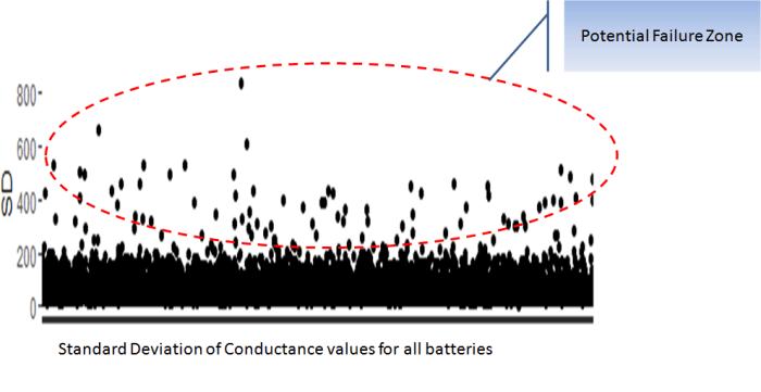
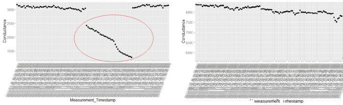


 The above is a plot depicting standard deviation of conductance for all batteries. Now what might be of interest to us is the red zone which we can call the “Potential failure Zone”. The potential failure zone consists of those batteries whose conductance values show high standard deviation. Batteries with failing health are likely to exhibit large fall in conductance and as a corollary their values will also show higher standard deviation. This implies that the samples of batteries which have higher probability of failure will in all likelihood be from this failure zone. However to ascertain this hypothesis we will have to dig deep into batteries in the failure zone and look for patterns which might differentiate them from normal batteries. Another objective to dig deep is also to elicit clues from the underlying patterns on what features to include in the predictive model. We will discuss more on the feature extraction when we discuss about feature engineering. Now let us come back to our discussion on digging deep into the failure zone and ferreting out significant patterns. It has to be noted that in addition to the samples in the failure zone we will also have to observe patterns from the normal zone to help separate wheat from the chaff . Intuitions derived by observing different patterns would become vital during feature engineering stage.
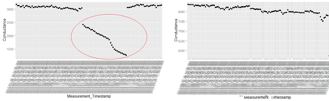
 .
.


 In the last few posts, where we discussed


