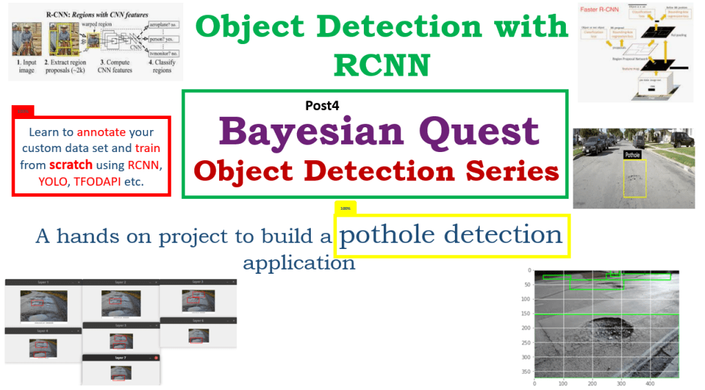
This is the fifth post of the series were we build a pothole detection application. We will be using multiple methods through out this series which includes computer vision techniques using Opencv, annotating images using LabelImg, mastering Tensorflow object detection API, Training objection detection using transfer learning, Object detection on video etc. This series will be split across 8 posts.
1. Introduction to object detection
2. Data set preparation and annotation Using LabelImg
3. Building your object detection model from scratch using Image pyramids and sliding window
4. Building your road pothole detector using RCNN
5. Building your road pothole detector using YOLOV5 ( This Post )
6. Building you road pothole detector using Tensorflow object detection API
7. Building your video analytics application for detecting potholes
8. Deploying your video analytics application for detection of potholes
In this post we will build our pothole detector using YOLO-V5. Let us start our process.
Introduction to YOLO
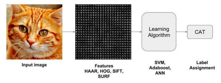
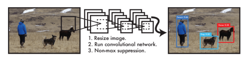
YOLO which stands for “You only look once” is one of the most popular object detector in use. The algorithm is designed in a way that by a single pass of forward propagation the network would be able to generate predictions. YOLO achieves very high accuracy and works really well in real time detection.
YOLO take a batch of images of shape (m, 224,224,3) and then outputs a list of bounding boxes along with its confidence scores and class labels, (pc,bx,by,bw,bh,c).
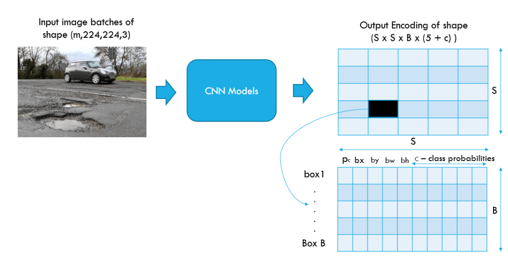
The output generated will be a grid of dimensions S x S ( eg. 19 x 19 ) with each grid having a set of B anchor boxes. Each box will contain 5 basic dimensions which include a confidence score and 4 bounding box information. Along with these 5 basic information, each box will also have the probabilities of the classes. So if there are 10 classes, there will be in total 15 ( 5 + 10) cells in each box. Let us look at the process in detail
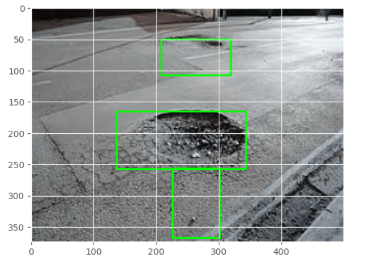
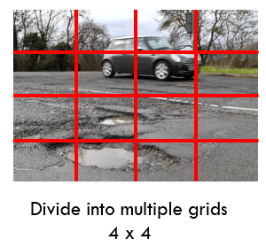
The start of the process in YOLO is to divide the image into a S x S grids. Here S can be any integer value. For our example let us take S to be 4.
Each cell would predict B boxes with a confidence score. Again B can be decided based on the number of objects that can be contained in a cell. An important condition that needs to be met is that the center of the box should be within the cell. These B boxes are called the anchor boxes.
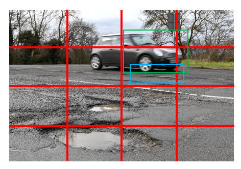
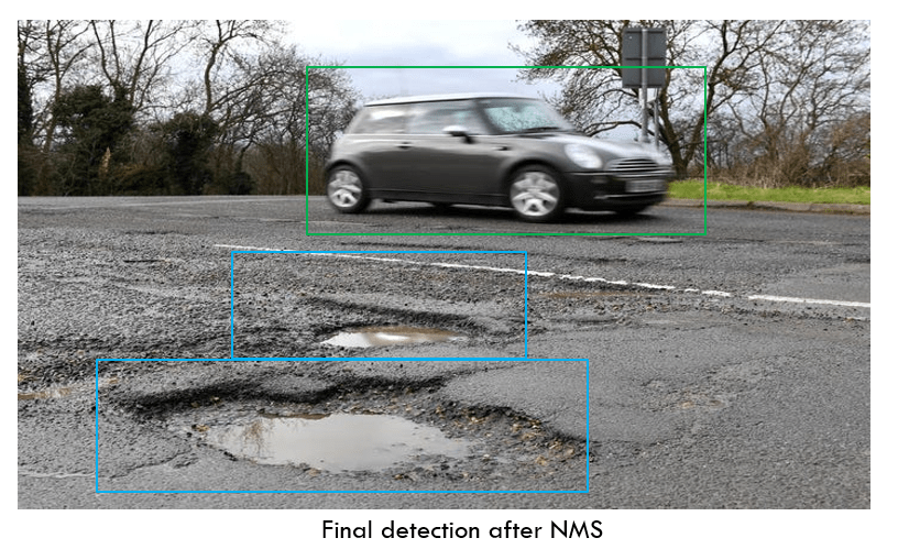
In our case, let us consider that B = 2. So each cell will predict 2 boxes where there is some probability of an object. Let us take the grid as shown in the above picture, where two boxes are predicted. That cell was able to detect a pothole and the car, and we can also see that the center of the boxes are also in the same cell. This process of predicting boxes happens for every cell within the image. In the course of this step multiple overlapping boxes will be predicted across all the grids of the image.

Along with the boxes and confidence scores a class probability map is also predicted. A class probability map gives the likelihood of the presence of a class in each of the cell. For example, vehicle in cell 2,3,4 …. and pothole in cell 9,10,11,…. etc.
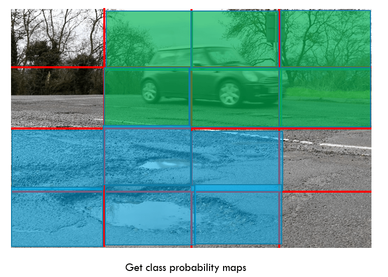
The class probability maps enables the network to assign a class map to each of the bounding boxes. Finally non maxima suppression is applied to reduce the number of overlapping boxes and get the bounding boxes of only the objects we want to classify.
Having seen an overview of the end to end process, let us look at the output or predictions from each cell. Let us look specifically at a cell shown in the image below.
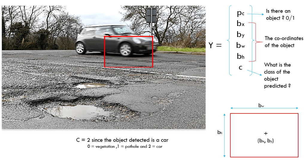
Each of the cells predicts a confidence score, which indicates if there is an object in the cell. Along with the confidence score, the bounding boxes of the object and the class of the object is also predicted. The class label can be an integer like 2 or 1 or it could be a one hot encoding representation of the predicted class ( eg. [0,0,1] ).
Having got an overview of YOLO , let us get into the implementation details.
Implementation of YOLO-V5
We will be managing the process through a Jupyter notebook. As this is a pre-trained model, we will not have too many activities to control in the process. The total process of implementation would have the following steps
- Downloading the YOLO V5 model files
- Preparing the annotated files
- Preparing the train, validation and test sets
- Implementing the training process
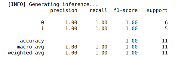
- Executing the inference process using the trained model
We will be training our custom Yolo model using Pytorch. Let us start by importing all the packages we require.
import pandas as pd
import os
import glob
from PIL import Image, ImageDraw
import numpy as np
import matplotlib.pyplot as plt
import random
from sklearn.model_selection import train_test_split
import shutil
import torch
from IPython.display import Image  # for displaying images
import os
import random
import shutil
import PIL
In the first step we clone the official repository of YOLOV5. We do it from the terminal or we can execute the same from Jupyter notebook too. Let us clone the repository from the Jupyter notebook.
! git clone https://github.com/ultralytics/yolov5
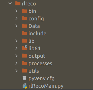
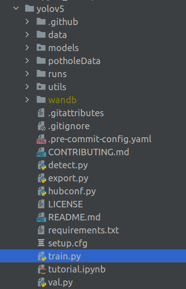
After the clone we will find a folder of YOLOV5 created in the folder where the Jupyter notebook resides.

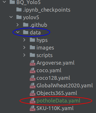
The Yolov5 folder will have many more default folders under it. The folder structure will look like the below.

Please note that the folder ‘potholeData‘ will not be part of the default yolov5 folder. This folder will be created by us in a moment from now.
We will now change directory to the yolov5 folder we created now. All the processes we will execute will be from that folder.
Next we will prepare the annotated file
Prepare annotation file
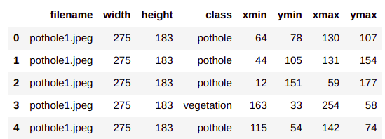
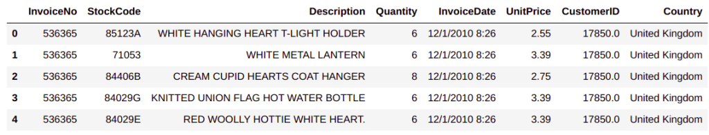
To prepare the annotated file we will use the annotation csv file which we created in post2. Let us first read the file
# Reading the csv file
pothole_df = pd.read_csv('BayesianQuest/Pothole/pothole_df.csv')
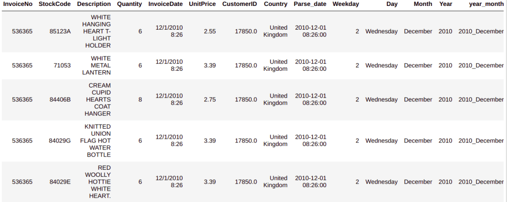
pothole_df.head()

Now we will create a class map, which is a dictionary which maps each of our classes to an integer value.
# First get the list of all classes
classes = pothole_df['class'].unique().tolist()
# Create a dictionary for storing class to ID mapping
classMap = {}

for i,cls in enumerate(classes):
    # Map a class name to an integet ID
    classMap[cls] = i

classMap

Next we will extract the bounding box information of the images from excel sheet in a specific format which is required for YoloV5. We also need to store the images and the annotation files ( labels ) in specific folders. Let us create the folders before we extract the bounding box information.
# Create the main data folder
!mkdir potholeData
# Create images and labels data folders
!mkdir potholeData/images
!mkdir potholeData/labels
# Create train,val and test data folders for both images and labels
!mkdir potholeData/images/train potholeData/images/val potholeData/images/test  potholeData/labels/train potholeData/labels/val potholeData/labels/test
After creation of these folders, our folder structure will look like the following

Now that we have created the data folders, let us start extracting the bounding box information. To do that we need to iterate through all the images we have and then get the bounding information in a .txt format, as required by YoloV5. Let us look at the code to do that.
# Creating the list of images from the excel sheet
imgs = pothole_df['filename'].unique().tolist()
# Loop through each of the image
for img in imgs:
    boundingDetails = []
    # First get the bounding box information for a particular image from the excel sheet
    boundingInfo = pothole_df.loc[pothole_df.filename == img,:]
    # Loop through each row of the details
    for idx, row in boundingInfo.iterrows():
        # Get the class Id for the row
        class_id = classMap[row["class"]]
        # Convert the bounding box info into the format for YOLOV5
        # Get the width
        bb_width = row['xmax'] - row['xmin']
        # Get the height
        bb_height = row['ymax'] - row['ymin']
        # Get the centre coordinates
        bb_xcentre = (row['xmin'] + row['xmax'])/2
        bb_ycentre = (row['ymin'] + row['ymax'])/2
        # Normalise the coordinates by diving by width and height
        bb_xcentre /= row['width']
        bb_ycentre /= row['height']
        bb_width    /= row['width']
        bb_height   /= row['height']
        # Append details in the list
        boundingDetails.append("{} {:.3f} {:.3f} {:.3f} {:.3f}".format(class_id, bb_xcentre, bb_ycentre, bb_width, bb_height))
    # Create the file name to save this info
    file_name = os.path.join("potholeData/labels", img.split(".")[0] + ".txt")
    # Save the annotation to disk
    print("\n".join(boundingDetails), file= open(file_name, "w"))
In line 2, we list down all the image ids from the csv file and then iterate through each of the image ids in line 4
We initialize a list in line 5 to capture the bounding box information and the get the bounding box information for the iterated image in line 7.
The bounding box information for each image is iterated through in line 9 and then we extract the class id in line 11 using the classMap dictionary we created.
From lines 14 -19, the bounding box information is extracted. When we created the annotations in post 2, we extracted the co-ordinates of the top left corner and the bottom right corner. However Yolo requires the width, height and the co-ordinates of the center of the image. In these lines we convert the coordinates to what is required by Yolo.
Lines 21-24 , co-ordinates are normalized by diving it by the width and height of the image and these coordinates are written to a text format in line 28.
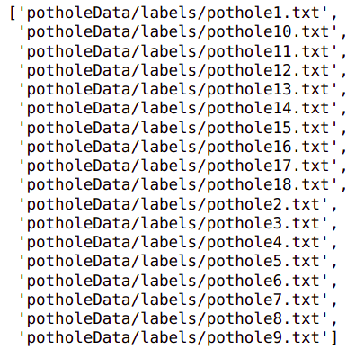
After executing this step you will be able to see the annotations as txt files in the labels folder.

Having completed the annotation of the data, let us prepare the train, test and validation sets.
Preparing the train, test and validation sets
To train the Yolo model, we need all the train, test & validation images and annotation text files in the respective folders which we created ( eg : ‘/images/train’, ‘labels/train’ etc). In this section we will list down the paths of the images and annotation texts, split the paths to train, test and validation sets and then copy the images and annotation files to the right folders. Let us see how we do that.
First let us get the paths of the annotation text files and images
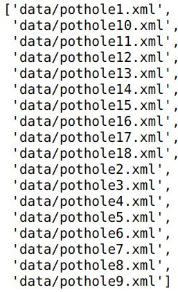
# Get the list of all annotations
annotations = glob.glob('potholeData/labels' + '/*.txt')
annotations
# Get the list of images from its folder
imagePath = '/media/acer/7DC832E057A5BDB1/JMJTL/Tomslabs/BayesianQuest/Pothole/data/annotatedImages'
images = glob.glob(imagePath + '/*.jpeg')
images

Please note to change the path of the images to the correct path where your images are placed in your system.
Next we sort the images and annotation files and the split the data into train/test/val sets
# Sort the annotations and images and the prepare the train ,test and validation sets
images.sort()
annotations.sort()

# Split the dataset into train-valid-test splits
train_images, val_images, train_annotations, val_annotations = train_test_split(images, annotations, test_size = 0.2, random_state = 123)
val_images, test_images, val_annotations, test_annotations = train_test_split(val_images, val_annotations, test_size = 0.5, random_state = 123)
Now we will create a utility function to copy the actual files from the source files to the destination folders.
#Utility function to copy images to destination folder
def move_files_to_folder(list_of_files, destination_folder):
    for f in list_of_files:
        try:
            shutil.copy(f, destination_folder)
        except:
            print(f)
            assert False
Let us now copy the files using the above utility function
# Copy the splits into the respective folders
move_files_to_folder(train_images, 'potholeData/images/train')
move_files_to_folder(val_images, 'potholeData/images/val/')
move_files_to_folder(test_images, 'potholeData/images/test/')
move_files_to_folder(train_annotations, 'potholeData/labels/train/')
move_files_to_folder(val_annotations, 'potholeData/labels/val/')
move_files_to_folder(test_annotations, 'potholeData/labels/test/')
Now you will be able to see the images and annotation text files in the respective folders

Now we are ready to start the training.
Training the model
Before initiating the training process we have to create a special file called .yaml file which contains information about the paths to the train, test and val folders and also the class labels. Let us create the yaml file first. Open your text editor and name it 'potholeData.yaml' and copy the following code in it.
train: /BayesianQuest/Pothole/yolov5/potholeData/images/train/
val:  /BayesianQuest/Pothole/yolov5/potholeData/images/val/
test: /BayesianQuest/Pothole/yolov5/potholeData/images/test/

# number of classes
nc: 4

# class names
names: ["pothole","vegetation", "sign","vehicle"]
Please note that for the first three lines, you need to give the full path to your images/train, images/val and images/test folder. The number of class names should be in the exact order in which we have defined the classMap dictionary earlier. You need to save this .yaml file in the data folder
Now its time to start the training. To start the training you need to enter the following command on the Jupyter notebook. Alternatively you can also run the same command on the terminal
!python train.py --img 640 --cfg yolov5m.yaml --hyp data/hyps/hyp.scratch-med.yaml --batch 4 --epochs 500 --data potholeData.yaml --weights yolov5m.pt --workers 4 --name yolo_pothole_det_m
Let us understand each of these parameters we give to initiate training
train.py : This is the training file which comes with the code when we clone the folder. This file contains all the methods to run the training.
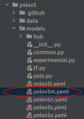
img : This is the dimension of the image
cfg : This is the configuration file which defines the model architecture. This file would be available in the folder yolov5/models as shown below.
hyp : These are the hyperparameters for the model which are available in the data/hyp folder

batch : This is the batch size, which you define based on the number of images you have
epochs : Number of training epochs
data : This is the yaml file which we created which has the path to the train/test/val files and also class information.
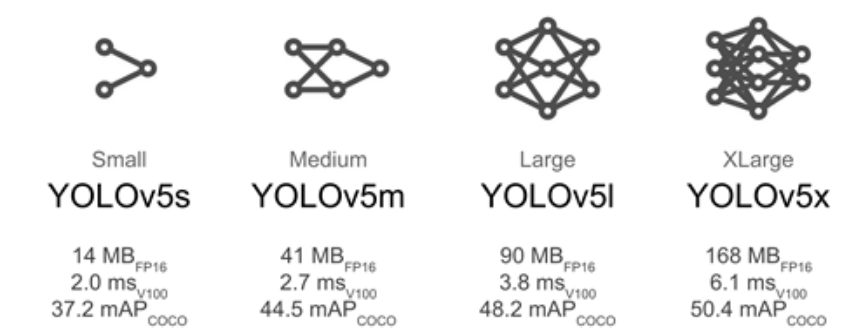
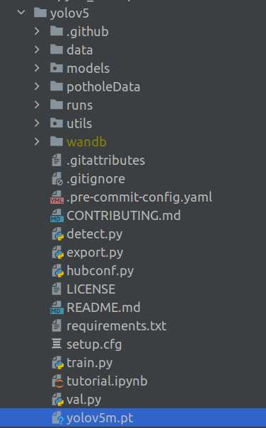
weights : These are the pre-trained weights of the model which will be automatically downloaded as part of the script. There are three types of models, large, medium and small. These are denoted by the abbreviations 'm' in yolov5m.pt. Here we have selected the medium model. When you run the training process for the first time, this weights file gets downloaded into the yolov5 folder.
workers : This indicate the number of cores/threads which needs to be used for training.
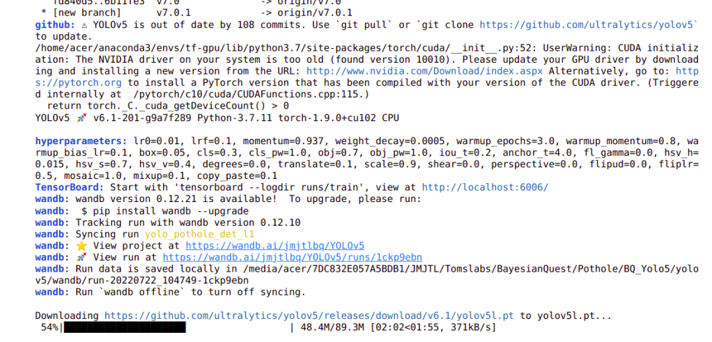
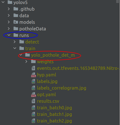
name : This is the name of the folder where the trained model and its checkpoints are stored. When you run the training command line, you will notice that a folder will be created with the same name as shown below. This will be inside a folder called ‘runs‘, which will be created inside the yolov5 folder.
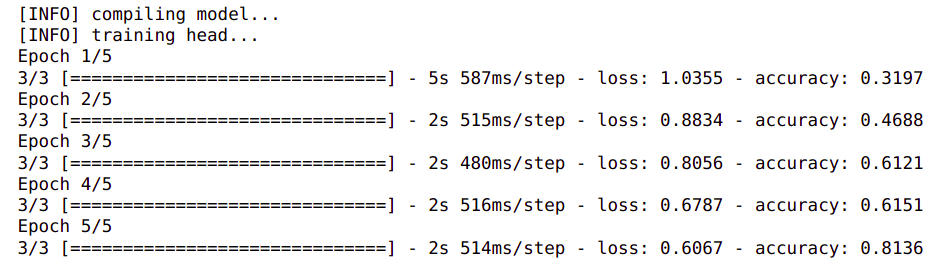
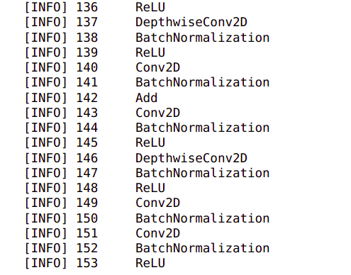
Once the training command is executed, you will see output similar to below on the screen

The training is a time consuming activity and can be visualized on Tensorboard by entering the following command on a terminal. Please note that the terminal should be pointing to the yolov5 folder. The log details required to run Tensorboard will be available in runs/train folder

Once this command is executed, you will find the following output and will be able to visualize the training run on the browser in the following url http://localhost:6006/
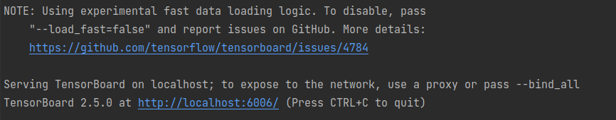
Once you open the browser you will find a similar output

Once the training is complete, the trained model weights will be stored in the — name folder you defined during the training process ( runs/train/yolo_pothole_det_m/weights/best.pt ). This weights would be used for your inference cycle.
Inference with the trained model
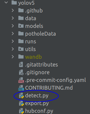
The inference will also be using a pre-defined script which comes with the Yolov5 package. Inference can be initiated using the following command on the Jupyter notebook.
!python detect.py --source potholeData/images/val/ --weights runs/train/yolo_pothole_det_m/weights/best.pt --max-det 3 --conf-thres 0.005 --classes 0 --name yolo_pothole_det_test_m1
Alternately you can also run the same on the terminal as below

Let us go through each of the parameters
detect.py : This is the file used for inference which is available in the yolov5 folder
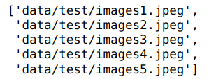
source : This is the path where the validation images are kept for inference. You can point this to any folder where you have your images which needs to be predicted on.
weights : This is the path to the weight of the checkpointed model we trained. These weights will be used for inference.
max-det : This is a parameter to define how many objects you want to be detected in an image.
conf-thres : This is a confidence threshold above which you want the predictions to be visualized.
classes : This is a parameter to filter the classes we want to be displayed. In the example we have defined only the pothole class ( 0 ). If we want objects of other classes to be defined, those class ids need to be represented with this parameter. ( eg. –classes 0 3 )
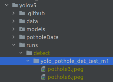
name : This is the path where the detected objects will exist. You will find a folder with the name you defined in the following folder.
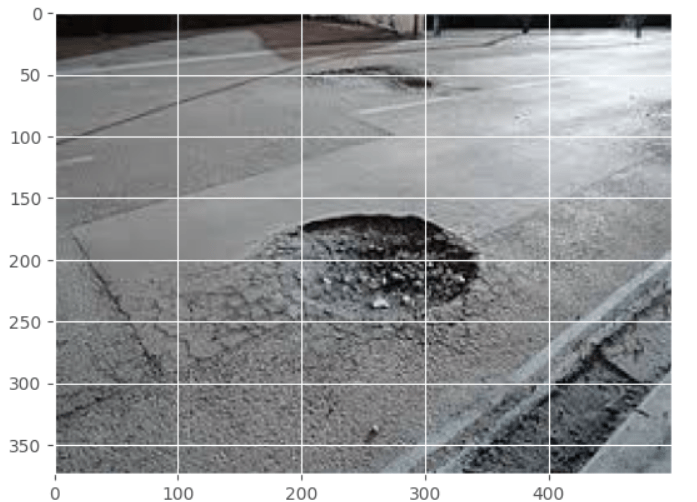
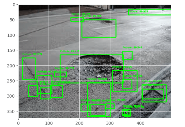
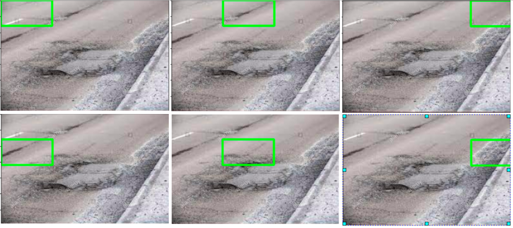
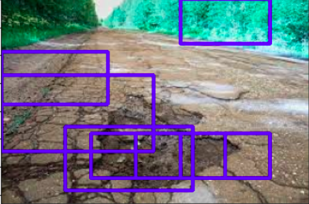
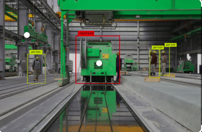
Let us look at some of the images we have predicted


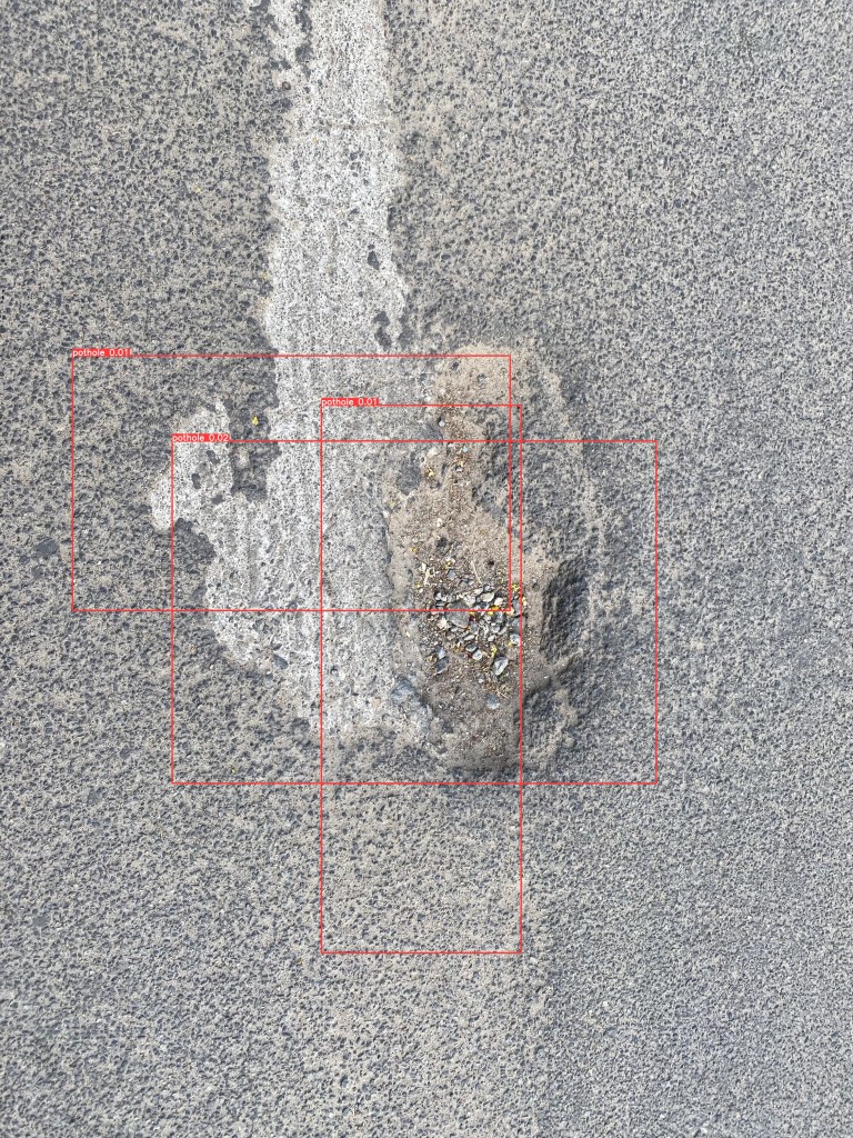
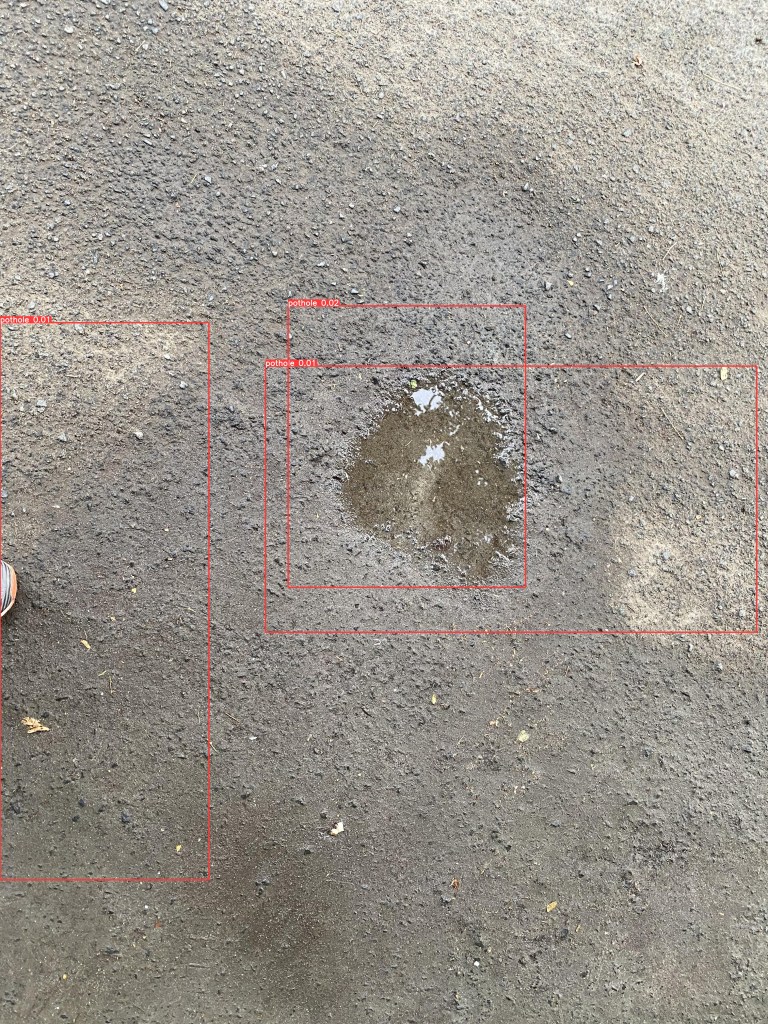
We can see that the bounding boxes have localized well. We should note that the number of images we used were very less and still we got some good results. With more images, we will be able to get superior results.
With this we have come to the end of object detection using YOLOV5. Let us quickly recap what we have achieved in this post.
- Downloaded the YOLOV5 scripts into our local folder
- Learned how to pre-process the data for custom training using YOLOV5.
- Trained the model and verified the best model
- Used the best model to do inference on our test images.
We have come a long way and are now adept at training and doing inference using an advanced model like YOLOV5. I am sure this will be another great tool with which you could do your object detection project.
What Next ?
Having seen an advanced method like YOLOV5, we will now proceed to learn to use a great tool from Tensorflow called the Tensorflow Object Detection API ( TFODAPI ). Using this API we would be able to build different types of object detection models. We will cover pothole detection using TFODAPI in the next post . Watch this space for more.
To be notified of the next post please subscribe to this blog post .You can also subscribe to our Youtube channel for all the videos related to this series.
You can also access the code base for this series from the following git hub link
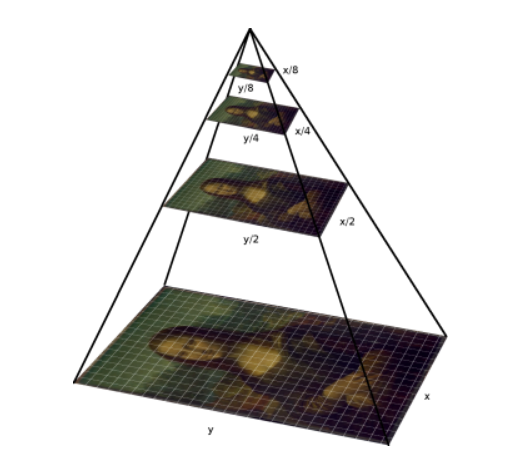
Do you want to Climb the Machine Learning Knowledge Pyramid ?
Knowledge acquisition is such a liberating experience. The more you invest in your knowledge enhancement, the more empowered you become. The best way to acquire knowledge is by practical application or learn by doing. If you are inspired by the prospect of being empowered by practical knowledge in Machine learning, subscribe to our Youtube channel
I would also recommend two books I have co-authored. The first one is specialized in deep learning with practical hands on exercises and interactive video and audio aids for learning

This book is accessible using the following links
The Deep Learning Workshop on Amazon
The Deep Learning Workshop on Packt
The second book equips you with practical machine learning skill sets. The pedagogy is through practical interactive exercises and activities.

This book can be accessed using the following links
The Data Science Workshop on Amazon
The Data Science Workshop on Packt
Enjoy your learning experience and be empowered !!!!