III : Build and Deploy Data Science Products : Looking under the hood of Machine translation model – LSTM Forward Propagation

Source : How stuff works

“Look deep into nature and you will understand everything better”

Albert Einsteen

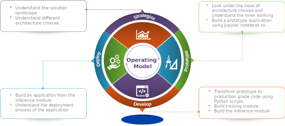
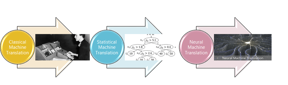
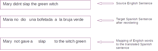
This is the third part of our series on building a machine translation application. In the last two posts we understood the solution landscape for machine translation and also explored different architecture choices for sequence to sequence models. In this post we take a deep dive into the dynamics of the model we use for machine translation, LSTM model. This series consists of 8 posts.

  1. Understand the landscape of solutions available for machine translation
  2. Explore sequence to sequence model architecture for machine translation.
  3. Deep dive into the LSTM model with worked out numerical example.( This post)
  4. Understand the back propagation algorithm for a LSTM model worked out with a numerical example.
  5. Build a prototype of the machine translation model using a Google colab / Jupyter notebook.
  6. Build the production grade code for the training module using Python scripts.
  7. Building the Machine Translation application -From Prototype to Production : Inference process
  8. Build the machine translation application using Flask and understand the process to deploy the application on Heroku

Dissecting the LSTM network

I was recently reading the book ” The Agony and the Ecstacy’ written by Irving Stone. This book was about the Reniassence genius, master sculptor and artist Michelangelo. When sculptuing human forms, in his quest for perfection , Miehelangelo used to spent months dissecting dead bodies to understand the anotomy of human beings. His thought process was that unless he understood in detail how each fibre of human muscle work, it would be difficult to bring his work to life. I think his experience in dissecting and understanding the anatomy of the human body has had a profound impact on his masterpieces like Moses, Pieta,David and his paintings in the Sistine Chapel.

Michaelangelo’s Moses,Pieta, David & Sistine chapel frescos

I too believe in that philosophy of getting a handle on the inner working of algorithms to really appreciate how they can be used for getting the right business outcomes. In this post we will understand the LSTM network in depth and explore its therotical underpinnings. We will see a worked out example of the forward pass for a LSTM network.

Forward pass of the LSTM

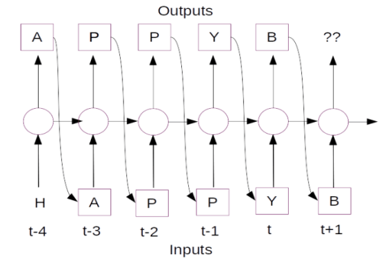
Let us learn the dynamics of the forward pass of LSTM with a simple network. Our network has two time steps as represented in the below figure. The first time step is represented as 't-1' and the subsequent one as time step 't'

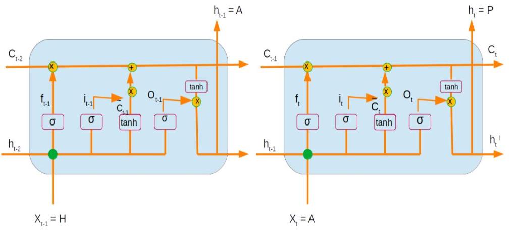
Let us try to understand each of the terms in the above network. A LSTM unit receives as its input the following

  1. c<t-2> : The cell state of the previous time step
  2. a<t-2> : The output from the previous time step
  3. x<t-1> : The input of the present time step

The cell state is the unit which is responsible for trasmitting the context accross different time steps. At each time step certain add and forget operations happens to the context transmitted from the previous time steps. These Operations are controlled through multiple gates. Let us understand each of the gates.

Forget Gate

The forget gate determines what part of the input have to be introduced into cell state and what needs to be forgotten. The forget gate operation can be represented as follows

Ґf = sigmoid(Wf*[ xt ] + Uf * [ at-1 ] + bf)

There are two weight parameters ( Wf and Uf ) which transforms the input ( xt ) and the output from the previous time step ( at-1) . This equation can be simplified by concatenating both the weight parameters and the corresponding xt & at vectors to a form given below.

Ґf = sigmoid(Wf *[xt , at-1] + bf)

Ґf is the forget gate

Wf is the new weight matrix got by concatenating [ Wf , Uf]

[xt , at-1]is the concatenation of the current time step input and the previous time step output from the

bf is the bias term.

The purpose of the sigmoid function is to quash the values within the bracket to act as a gate with values between 0 & 1 . These gates are used to control the flow of information. A value of 0 means no information can flow and 1 means all information needs to pass through. We will see more of those steps in a short while.

Update Gate

Update gate equation is similar to that of the forget gate . The only difference is the use of a different weight for this operation.

Ґu = sigmoid(Wu *[xt , at-1] + bu)

Wu is the weight matrix

Bu is the bias term for the update gate operation

All other operations and terms are similar to that in the forget gate

Input activation

In this operation the input layer is activated using a tanh non linear activation.

C~ = tanh(Wc *[x , a] + bc)

C~ is the input activation

Wc is the weight matrix

bc is the bias term which is added.

operation converts the terms within the bracket to values between -1 & 1 . Let us take a pause and analyse why a sigmoid is used for the gate operations and tanh used for the input activation layers.

The property of sigmoid is to give an output between 0 and 1. So in effect after the sigmoid gate, we either add to the available information or do not add any thing at all. However for the input activation we also might need to forget some items. Forgetting is done by having negative values as output. tanh layer ranges from -1 to 1 which you can see have negative values. This will ensure that we will be able to forget some elments and remember others when using the tanh operation.

Internal Cell State

Now that we have seen some of the building block operations, let us see how all of them come together. The first operation where all these individual terms come together is to define the internal cell state.

We already know that the forget and update gates which have values ranging between 0 to 1, act as controllers of information. The forget gate is applied on the previous time step cell state and then decides which of the information within the previous cell state has to be retained and what has to be eliminated.

Ґf * C<t-1>

The update gate is applied on the input activation information and determines which of these information needs to be retained and what needs to be eliminated .

Ґu * C~

These two informations block i.e the balance of the previous cell state and the selected information of the input activation are combined together to form the current cell state. This is represented in the equation as below.

C<t> = Ґu * C~ + Ґf * C<t-1>

Output Gate

Now that the cell state is defined it is time to work on the output from the current cell. As always, before we define the output candidates we first define the decision gate. The operations in the output gate is similar to the forget gate and the update gate .

Ґo = sigmoid(Wo *[x , a] + bo)

Wo is the weight matrix

Bo is the bias term for the update gate operation

Output

The final operation within the LSTM cell is to define the output layer. The output candidates are determined by carrying out a tanh() operation on the internal cell state. The output decision gate is then applied on this candidate to derive the output from the network. The equation for the output is as follows

a<t> = tanh(C<t>) * Ґo

In this operation using the tanh operation on the cell state we arrive at some candidates to be forgotten ( -ve values) and some to be remembered or added to the context. The decision on which of these have to be there in the output is decided by the final gate, output gate.

This sums up the mathematical operations within LSTM. Let us see these operations in action using a numerical example.

Dynamics of the Forward Pass

Now that we have seen the individual components of a LSTM let us understand the real dynamics using a toy numerical examples.

The basic building block of LSTM like any neural network is its hidden layer, which comprises of a set of neurons. The number of neurons within its hidden unit is a hyperparameter when initializing a LSTM. The dimensions of all the other components of a LSTM depends on the dimension of the hidden unit. Let us now define the dimensions of all the components of the LSTM.

ComponentDescriptionDimension of the component
LSTM hidden unitSize of the LSTM unit ( No of nuerons of the hidden unit)(n_a)
mNumber of examples(m)
n_xSize of inputs(n_x)
C<t-1>Dimension of previous cell state(n_a , m)
a<t-1>Dimensions of previous output(n_a , m)
x<t>Current state input(n_x , m)
[ x<t> , a<t-1> ]Concatenation of output of previous time step and current time step input(n_x + n_a, m)
Wf, Wu, Wc, WoWeights for all the gates(n_a , n_x + n_a)
bf bu bc b0Bias term for all operations(n_a ,1)
WyWeight for the output(n_y , n_a)
byBias term for the output(n_y ,1)

Let us now look at how the dimensions of the different outputs evolve after different operations within the LSTM .

Please note that when we do matrix multiplications with two matrices of size ( a,b) * (b,c) we get an output of size (a,c)
ComponentOperationDimensions
Ґf : Forget gatesigmoid(Wf * [x , a] + bf)(n_a, n_x + n_a) * (n_x + n_a ,m) + (n_a,1) = > (n_a , m).
Sigmoid is applied element wise and therefore dimension doesn’t change.
* : denotes matrix multiplication
Ґu: Update gatesigmoid(Wu *[x , a] + bu)(n_a, n_x+n_a ) * (n_x+n_a,m) + (n_a,1) = > (n_a , m)
C~: Input activationtanh(Wc *[x , a] + bc)(n_a, n_x + n_a) * (n_x + n_a , m) + (n_a, 1) = > (n_a, m).
Ґo : Output gate(Wo *[x , a] + bo)(n_a, n_x+n_a ) * (n_x + n_a ,m) + (n_a,1) = > (n_a,m)
C<t> : Current stateҐu x C~ + Ґf x C<t-1>(n_a, m) x (n_a, m) + (n_a, m) x (n_a, m) = > (n_a, m)
x: denotes element wise multiplication
a<t> : Output at current time steptanh(C<t>) x Ґo(n_a, m) x (n_a, m) => (n_a, m).

Let us do a toy example with a two time step network with random inputs and observe the dynamics of LSTM.

The network is as defined below with the following inputs for each time steps. We also define the actual outputs for each time step. As you might be aware the actual output will not be relevant during the forward pass, however it will be relevant during the back propogation phase.

Toy example with LSTM

Our toy example will have two time steps with its inputs (Xt) having two features as shown in the figure above. For time step 1 the input is Xt-1 = [0.4,0.3] and for time step 2 the input is Xt = [0.2,0.6]. As there are two features, the size of the input unit is n_x = 2. Let us tabulate these values

VariableDescriptionValuesDimension
X t-1Input for the first time step[0.4, 0.3](n_x , m)
= > (2 ,1)
XtInput for the second time step[0.2, 0.6](n_x , m)
= > (2 ,1)

For simplicity the hidden layer of the LSTM has only one unit which means that n_a = 1. For the first time step we can assume initial values for the cell state Ct-2 and output from previous layers at-2 as ‘0’.

VariableDescriptionValuesDimension
Ct-2Initial cell state[0](n_a , m) = > (1 ,1)
at-2Initial output from previous cell[0](n_a , m) = > (1 ,1)

Next we have to define the values for the weights and biases for all the gates. Let us randomly initialize values for the weights. As far as the weights are concerned, what needs to be carefully defined are the dimensions of the weights. In the earlier table where we defined the dimensions of all the components we defined the dimension of the weights as (n_a , n_x + n_a). But why do the weights be with these dimensions ? Let us dig deeper.

From our earlier discussions we know that the weights are used to get the sigmoid gates which are multiplied element wise on the cell states. For example

Ct = Ґu * C~ + Ґf * Ct-1

or

at = tanh(Ct) * Ґo.

From these equations we see that the gates are multiplied element wise to the cell states. To do an element wise multiplication, the gates have to be of the same dimensions as the cell state, i.e. (n_a, m). However, to derive the gates, we need to do a dot product of the initialised weights with the concatenation of previous cell state and the input vector [n_x+n_a]. Therefore to get an output dimension of (n_a, m) we need to have the weights with dimensions of (n_a , n_x + n_a) so that the equation of the gate ,Ґf = sigmoid(Wf *[x , a] + bf), generates an output of dimension of (n_a ,m ). In terms of matrix multiplication dynamics this equation can be represented as below

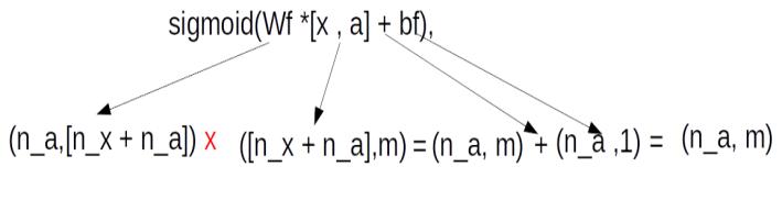
Having seen how the dimensions are derived, let us tabulate the values of weights and its biases .Please note that the values for all the weight matrices and its biases are randomly initialized.

WeightDescriptionValuesDimension
Wf,Forget gate Weight[-2.3 , 0.6 , -0.13 ]
[n_a , n_x + n_a] => (1,3)
bfForget gate bias[0.51][n_a] => 1
WuUpdate gate weight[1.51 ,-0.61 , 1.31][n_a , n_x + n_a] => (1,3)
buUpdate gate bias[1.30][n_a] => 1
Wc,Input activation weight[0.82,-0.57,-0.13][n_a , n_x + n_a] => (1,3)
bcInternal state bias[-0.57][n_a] => 1
WoOutput gate weight[-0.75 ,-0.95 , -0.34][n_a , n_x + n_a] => (1,3)
b0Output gate bias[-0.46][n_a] => 1

Having defined the initial values and the dimensions let us now traverse through each of the time steps and unravel the numerical example for forward propagation.
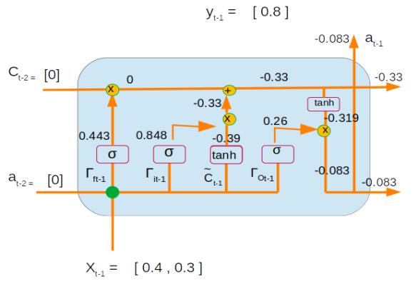
Time Step 1 :

Inputs : X t-1 = [0.4, 0.3]

Initial values of the previous state

at-2= [0] ,

Ct-2 = [0]

Forget gate => Ґf = sigmoid(Wf *[x , a] + bf) =>

= sigmoid( [-2.3 , 0.6 , -0.13 ] * [0.4, 0.3, 0] + [0.51] )

= sigmoid(((-2.3 * 0.4) + (0.6 * 0.3) + (-0.13 * 0 )) + 0.51)

= sigmoid(-0.23) = 0.443

Please note  sigmoid (-0.23) = 1/(1 + e(-(-0.23))

Update gate => Ґu = sigmoid(Wu *[x , a] + bu) =>

= sigmoid( [1.51 ,-0.61 , 1.31] * [0.4, 0.3, 0] + [1.30] )

= sigmoid((1.51 * 0.4) + (-0.61 * 0.3) + (1.31 * 0 ) + 1.30)

= sigmoid(1.721) = 0.848

Input activation => C~ = tanh(Wc *[x , a] + bc)

= tanh( [0.82,-0.57,-0.13] * [0.4, 0.3, 0] + [-0.57] )

= tanh (((0.82 * 0.4) + (-0.57 * 0.3) + (-0.13 * 0 )) + -0.57)

= tanh(-0.413) = -0.39

Please note tanh = ex – e-x / ( ex + e-x) where x = -0.413
= e-0.413 – e-(-0.413) / ( e-0.413 + e-(-0.413)) = -0.39

Output Gate => Ґo = sigmoid(Wo *[x , a] + bo)

= sigmoid( [-0.75 ,-0.95 , -0.34] * [0.4, 0.3, 0] + [-0.46] )

= sigmoid(((-0.75 * 0.4) + (-0.95 * 0.3) + (-0.34 * 0 )) + -0.46)

= sigmoid(-1.045)= 0.26

We now have all the components required to calculate the internal state and the outputs

Internal state => Ct-1 = Ґu * C~ + Ґf * Ct-2

= 0.848 * -0.39 + 0.443 * 0

= -0.33

Output => at-1 = tanh(Ct-1) * Ґo

= tanh(-0.33) * 0.26 = -0.083

Let us now represent all the numerical values for the first time step on the network.

With the calculated values of time step 1 let us proceed to calculating the values of time step 2
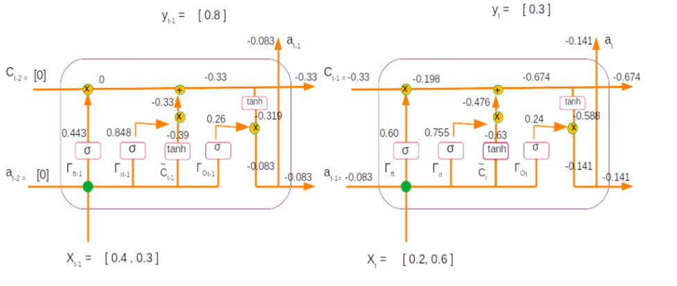
Time Step 2:

Inputs : Xt = [0.2, 0.6]

Values of the previous state output and cell states

at-1 = [-0.083]

Ct-1 = [-0.33]

Forget gate => Ґf = sigmoid(Wf *[xt , at-1] + bf) =>

= sigmoid( [-2.3 , 0.6 , -0.13 ] * [0.2, 0.6, -0.083] + [0.51] )

= sigmoid(((-2.3 * 0.2) + (0.6 * 0.6) + (-0.13 * -0.083 )) + 0.51)

= sigmoid(0.421) = 0.60

Update gate => Ґu = sigmoid(Wu *[xt , at-1] + bu) =>

= sigmoid( [1.51 ,-0.61 , 1.31] * [0.2, 0.6, -0.083] + [1.30] )

= sigmoid(((1.51 * 0.2) + (-0.61 * 0.6) + (1.31 * -0.083 )) + 1.30)

= sigmoid(1.13) = 0.755

Input activation => C~ = tanh(Wc *[xt , at-1] + bc)

= tanh( [0.82,-0.57,-0.13] * [0.2, 0.6, -0.083] + [-0.57] )

= tanh(((0.82 * 0.2) + (-0.57 * 0.6) + (-0.13 * -0.083 )) + -0.57)

= tanh(-0.737) = -0.63

Output Gate => Ґo = sigmoid(Wo *[x , a] + bo)

= sigmoid( [[-0.75 ,-0.95 , -0.34] * [0.2, 0.6, -0.083] + [-0.46] )

= sigmoid(((-0.75 * 0.2) + (-0.95 * 0.6) + (-0.34 * -0.083 )) + -0.46)

= sigmoid(-1.15178)= 0.24

Internal state => Ct = Ґu * C~ + Ґf * Ct-1

= 0.755 * -0.63 + 0.60 * -0.33

= -0.674

Output => at = tanh(Ct) * Ґo

= tanh(-0.674) * 0.24 = -0.1410252

Let us now represent the second time step within the LSTM unit

Second Time step

Let us also look at both the time steps together with all its numerical values

This sums a single forward pass for the LSTM. Once the forward pass is calculated the next step is to determine the error term and the backpropagating the error to determine the adjusted weights and bias terms. We will see those steps in the back propagation steps, which will be covered in the next post.

Go to article 4 of this series : Back propagation of the LSTM unit

Do you want to Climb the Machine Learning Knowledge Pyramid ?

Knowledge acquisition is such a liberating experience. The more you invest in your knowledge enhacement, the more empowered you become. The best way to acquire knowledge is by practical application or learn by doing. If you are inspired by the prospect of being empowerd by practical knowledge in Machine learning, I would recommend two books I have co-authored. The first one is specialised in deep learning with practical hands on exercises and interactive video and audio aids for learning

Deep Learning Workshop

This book is accessible using the following links

The Deep Learning Workshop on Amazon

The Deep Learning Workshop on Packt

The second book equips you with practical machine learning skill sets. The pedagogy is through practical interactive exercises and activities.

The Data Science Workshop Book

This book can be accessed using the following links

The Data Science Workshop on Amazon

The Data Science Workshop on Packt

Enjoy your learning experience and be empowered !!!!

II : Build and Deploy Data Science Products : Exploring Sequence to Sequence architecture for Machine Translation.

Source:curiodissey.org

“A sequence works in a way a collection never can”

George Murray

This is the second part of our series on building a machine translation application. In this post we explore sequence to sequence model architecture in greater depth. This series consists of the following eight posts.

  1. Understand the landscape of solutions available for machine translation
  2. Explore different sequence to sequence model architecture for machine translation.( This post)
  3. Deep dive into the LSTM model with worked out numerical example.
  4. Understand the back propagation algorithm for a LSTM model worked out with a numerical example.
  5. Build a prototype of the machine translation model using a Google colab / Jupyter notebook.
  6. Build the production grade code for the training module using Python scripts.
  7. Building the Machine Translation application -From Prototype to Production : Inference process
  8. Build the machine translation application using Flask and understand the process to deploy the application on Heroku

In the first part of this series we surveyed the solution landscape of machine translation applications and understood why sequence to sequence models are best suited for machine translation. In this post we will go little deeper and expore architectur choices for sequence to sequence models. We will specifically look at the encoder – decoder architecture which will be the specific architecture we will use for machine translation. We will also get a glimpse of the LSTM model which is the building block for the machine translation application we would be building.

We already know that the problem of machine translation entails deciphering sequence of words in a source language to predict a sequence of target language. For example if you look at the following input German sequence

Ich freue mich darauf, etwas über maschinelle Übersetzung zu lernen.
Which can be translated to 

I look forward to learning about machine translation

From these sequences we can observe the following.

  1. The length of input sequence and the length of the target sequence are different
  2. There is no one to one mapping between words from the input language to the target language
  3. There is dependence on the context which needs to be learned from the input language to get the best translation for the target language.

The inherent complexities like these in machine translation made models like multi layer perceptron ineffective for machine translation. The need of the hour was a model architecuture which was capable of looking accross sequences of words and understand the context of the source language to effectively translate to the target language. This is where Recurrent Neural Networks (RNNs) became popular for solving machine translation problems. Let us now take a deeper look at RNNs.

Recurrent Neural Networks ( RNNs)

RNN models which fall under the category of Sequence to sequence models are designed to learn the context of any input language. But why is learning the context important ? Let us understand this with a simple example.

Suppose we are predicting the next character in a sequence for the string “Happy B….”. We need to predict the next character after the letter ‘B’. For the time being let us assume that we are ignoring the word “Happy” falling before the letter B. In such a scenario the best bet would be to look for all the words which start with “B” and choose the word which is most frequent. Let us say the most frequent word starting with “B” is the word “Baby”. So the next character which will be predicted would be the letter “a”. Now let us imagine that we started looking at all the characters which preceeds B. Given the information about the preceeding charachters “H”,”A”,”P”,”P”,”Y” “B”, then the probability of predicting ‘i’ would be the highest since the word “Birthday” is the most likely word given the context “Happy B” . This is where the concept of context becomes very significant. Language translation depends a lot on the context and therefore there was the need to adopt an architecture where context was learned. Sequence to sequence models like RNNs became an obvious choice.

The dynamics of RNN can be represented as above. The circular nodes represents each time step in the sequence. Each of the time steps receives an input represetend as the arrow pointing upwards. In this context each letter in the string becomes the input at each time step. With each character input the output or the prediction is represented at the top. So given the letter ‘H’ the prediction is the letter ‘A’. Once the letter ‘A’ is predicted it becomes the next input and we need to predict the next letter given the context that we had the letter ‘H’ at the previous time step. At each time step we can also see that there is an arrow which points to the right. This is the information or context each time step passes on to the subsequent time step enabling it to predict contextually.

Unlike vanilla neural networks where each layer has a set of parameters, RNNs shares the same parameters accross all the time steps. Because the parameters are shared accross all time steps, the implementation of back propogation is a little different for the case of RNNs. The type of back propogation implemented in RNN is called Back propogation through time(BPTT). We will be covering the dynamics of BPTT with a toy example in the fourth blog of this series.

Earlier we saw that the RNN keeps the context of the previous time steps in memory and applies it when predicting for the time step in consideration. However in practice vanilla RNNs fails when it encounters large sequences. The parameters blow up or shrink to very small values in such cases. These scenarios are called exploding gradients and vanishing gradients respectively. So in practice a RNN can only leaverage few time steps to extract the context. To over come these shortcomings different variations sequence to sequence models are used. One such variation is the LSTM Long Short Term Memory network. We will be using the LSTM network in our application for machine translation. Let us first look at what an LSTM looks like.

Long Short Term Memory Network ( LSTM)

LSTMs, like vanialla RNNs, have the recurrent connections which entails that the context from the previous time steps are passed on to the current time step when generating an output. However we discussed in the previous section on RNN that they suffer from a major problem of exploding or vanishing gradients when encountered with long sequences. This shortcoming was overcome by building a memory block in LSTMs.

LSTM Network

The LSTM has three information sources,two from previous time steps and one from the current time step. The first one is the cell state denoted by ‘Ct’ . The cell state transmits the information about the context from the previous cell states. The second information which passes from the previous layer is its output denoted by ‘ht’. The third is the input for the present time step. In our context of predicting characters, the input from the time step t1 is the letter ‘H’. All these inputs get processed within the LSTM layer enabling it to have memory for longer sequences. We will be having a very detailed worked out example on the dynamics of LSTM in the next post.

An important part of building applications using sequence to sequence models is the selection of right architecture for the use case. Let us now look at different architecture choices for different use cases.

Network Architecture for Sequence to Sequence Models

There are different architecture choices for sequence to sequence models which varies according to the use case. Some of the prominent ones are

  • Many to one architecture

This is architecture is ideal for use cases like sentiment analysis where seeing a sequences of words in a string, predict a single output which in this case is the sentiment.

  • One to many architecture

This architecture is well suited for use cases like image translation. In such use cases, an image is provided as the input and a sequence of words describing the image is predicted as output. In this case there is one input and multiple outputs.

One to many architecture
  • Many to many architecture

This is the architecuture which is ideal for a use case like Machine translation. In this architecture, a sequence of words is given as input and the output is also another sequence of words. The below figure is a representation of German to English translation using the many to many architecture.

This architecture is also called Encoder-Decoder architecture. We will see the encoder-decoder architecture in greater depth during our prototype building phase.

Wrapping up

Its now time to wrap up our discussion on sequence to sequence. In this post we had an introduction on RNNs and in specific LSTM which we will be using for the machine translation application. We also looked at different types of architecture choices and identified the encoder-decoder architecture which will be more suited for our use case.

Having seen the conceptual level introduction of sequence to sequence models its time to look under the hood of the LSTM model. In the next post we will work out a toy numerical example and understand in greater depth how LSTM works.

Go to article 3 of the series : Deep dive into the LSTM model with worked out numerical example.

Do you want to Climb the Machine Learning Knowledge Pyramid ?

Knowledge acquisition is such a liberating experience. The more you invest in your knowledge enhacement, the more empowered you become. The best way to acquire knowledge is by practical application or learn by doing. If you are inspired by the prospect of being empowerd by practical knowledge in Machine learning, I would recommend two books I have co-authored. The first one is specialised in deep learning with practical hands on exercises and interactive video and audio aids for learning

Deep Learning Workshop

This book is accessible using the following links

The Deep Learning Workshop on Amazon

The Deep Learning Workshop on Packt

The second book equips you with practical machine learning skill sets. The pedagogy is through practical interactive exercises and activities.

The Data Science Workshop Book

This book can be accessed using the following links

The Data Science Workshop on Amazon

The Data Science Workshop on Packt

Enjoy your learning experience and be empowered !!!!

I : Build and Deploy Data Science Products : A Practical Guide to Building a Machine Translation Application.

Source : pintrest.com

“Investment in Knowledge pays the best dividend”

Benjamin Franklin

I was searching for a good quote to start this blog and that’s when I came across the above quote by Benjamin Franklin. I think the above quote best sums up what we are going to achieve in this series. We are going to invest our time in gaining an end to end perspective of a use case. We would be embarking on an exciting journey where we will get to experience a machine learning use case in its full glory, right from its theoretical base to building an application and deploying it. Our learning objectives are summed up in the below figure.

This journey is going to be a 8 post series. In this series we will take a use case, understand the solution landscape and its evolution, explore different architecture choices, look under the hood of the architecture to understand the nuts and bolts, build a prototype, convert the prototype into production ready code, build an application from the production ready code and finally understand the process for deploying the application .The use case we will be dealing with will be Machine Translation. By the end of the series you would have working knowledge on how to build and deploy a Machine translation application, which translates, German sentences into English. This series will comprise of the following posts.

  1. Understand the landscape of solutions available for machine translation ( This post)
  2. Explore sequence to sequence model architecture for machine translation.
  3. Deep dive into the LSTM model with worked out numerical example.
  4. Understand the back propagation algorithm for a LSTM model worked out with a numerical example.
  5. Build a prototype of the machine translation model using a Google colab / Jupyter notebook.
  6. Build the production grade code for the training module using Python scripts.
  7. Building the Machine Translation application -From Prototype to Production : Inference process
  8. Build the machine translation application using Flask and understand the process to deploy the application on Heroku

The first four posts lays the theoretical base and in the subsequent 4 posts we will see how the theory can be put to action. You can also watch videos of this series on Youtube.

Let us get started on this journey with an introduction to machine translation.

Introduction to Machine Translation

Language translation has always been a tough nut to crack. What makes it tough is the variations in structure and lexicon when one traverses from one language to the other. For this reason the problem of automated language translation or Machine translation has fascinated and inspired the best minds. Over the past decade some trailblazing advances have happened within this field. We have now reached a stage where machine translation has become quite ubiquitous. These technologies are now embedded in all our devices, mobiles, watches, desktops, tablets etc and have become an integral part of our every day life. A common example is the Google Translate service which has the capability to identify our input languge and subsequently translate it to multitudes of languages.

Machine translation technologies have transcended different approaches before reaching the state we are in at present. Let us take a quick look at the evolution of the solution landscape of machine translation.

Evolution of Solution landscape for Machine Translation

The journey to the current state of the art translation technologies tells a fascinating tale of the strides in machine learning.

The evolution of machine translation can be demarcated to three distinct phase. Let us look at each one of them and understand its distinct characteristics.

Classical Machine Translation

Classical machine translation methods relies heavily on linguisitc rules and deep domain knowledge to translate from a source language to a target language. There are three approaches under this method.

Direct Translation

“Direct translation is based on a large bilingual dictionary;each entry in the dictionary can be viewed as a small program whose job is to translate one word”

Source : Speech and Language processing : Daniel Jurafsky, James H Martin: 2nd Edition.

As the name suggests this method adopts a word-to-word translation of the source language to the target language. After the word to word translation a re-ordering of the translated words are required based on linguistic rules formulated between the source language and target language.

Let us look at an example

Example Source : Speech and Language processing : Daniel Jurafsky, James H Martin: 2nd Edition.

In the above example, the first two boxes represent the source English sentence and the final translated Spanish sentences respectively. The last box is a word to word mapping of the translated Spanish sentence to its English conuterpart. We can see how the word to word translation has been transformed by re-ordering to form a coherent sentence in the target language. These transformations are aided by comprehensive linguistic rules and deep domain knowledge.

Transfer Method

In the example we saw on direct translation method, we saw how the mapping of the English words for the translated Spanish sentence had a complete different ordering from the source English sentence. Every language has such structural charachteristics inherent in them. Transfer methods looks at tapping the structural differences between different language pairs.

Unlike the direct method where there is word to word tranlation followed by re-ordering, transfer methods relies on codification of the contrastive knowledge i.e difference between languages, for translation from the source to the target language. Similar to the direct method, this method also relies on deep domain knowledge and codification of complex rules governing language construction.

Interlingua Method

Image source : in.pinterest.com

The intelingua method works on a completely different approach to the word to word and contrastive translations methods we have already seen.

“The interlingua intuition is to treat translation as a process of extracting meaning of the input and then expressing the meaning in the target language.”

SOURCE : Speech and Language processing : Daniel Jurafsky, James H Martin: 2nd Edition.

The intelingua method resonates very closely to the process by which human translators work. When translating , a human translator understands the meaning of the source sentence and translate it to the target language so that the essence of the conversation is not lost. There might not be a word to word mapping of the source sentence and translated sentence. However the meaning would remain intact. This is the principle adopted in the intelingua methods. Like the other two methods in the classical approach, intelingua method also depends on the rich codification of rules and dictionaries

The classical machine translation methods were effective for a large set of use cases. However the classical methods relied on comprehensive set of rules and large dictionaries. Building such knowledge base was a mammoth task requiring specialised skills and expertise. The complexity increased many fold when designing systems able to handle translation of multiple languages. There was a need for an approach different from the domain intensive classical techniques. This led to the rise in popularity of the statistical methods in machine translation.

Statistical Machine Translation

When we explored the classical methods we understood the over dependence on domain knowledge in creating linguistic rules and dictionaries. However it was also a fact that no amount of domain knowledge was enough to handle the intricate nuances of languages. What if phrases, idioms and specialised usages in a language do not have any parallels in another language ? In such circumstances what a linguist would do is to go for the closest match given the source language.

This idea of selecting the most probable sentence in the target languge given a sentence in source language is what is leaveraged in statistical machine translation.

“This provides us with a hint to do Machine Translation. We can model the goal of translation as the production of an output that maximizes some value function that represents the importance of both faithfulness and fluency.”

SOURCE : SPEECH AND LANGUAGE PROCESSING : DANIEL JURAFSKY, JAMES H MARTIN: 2ND EDITION

Statistical methods builds probabilistic models that aims at maximizing the probability of the target sentence which best captures the essence of the source sentence. In probability terms we can represent this as

argmaxT P(T|S)

where T and S are the target and source languages respectively. The above form is the representation of a posterior probability as per Bayes Theorm. This is proportional to

= argmaxT P(S|T) * P(T)

The first term ( P(S|T) ) is called the translation model and can be interpreted as the likelihood of finding the source sentence given the target sentence. The second term P(T) is called the language model which represents the conditional probability of a word in the languge given some preceeding words.

The statistical model aims at finding the conditional probabilities of words within a corpora and using these probabilities find the best possible translation. Statistical machine translation models make use of large corpora or text available on the source and target languages. Eventhough statistical methods were effective, they also had some weaknesses. This method was predominantly focussed on phrases being translated thereby compromising the broder context of the target language. This method struggled when required to translate to a target language which was different in context from the source context. These shortcomings paved the way to advances in other methods which were more robust to retaining the context between the source and target languages.

Neural Machine Translation

Neural Machine Translation

Neural machine translation is a different approach where artifical neural networks are used for machine translation. In the statistical machine translation approaches we saw that it uses multiple components like the translation model and language model to do the translations.In NMT models the entire sentence is a single integrated model. In term of approach there isnt drastic deviations from the statistical approaches. However NMTs uses vector representations of words and sentences, which helps in retaining the context of the source and target sentences.

There are different approaches for machine translation using artificial neural networks. One of the earlier approach was to use a multi layer perceptron or a fully connected network for machine translation. However these models werent effective for large sequences of sentences.

Many shortfalls of the earlier approaches were addressed by the adoption of Recurrent Neural network models (RNNs) for machine translation. RNNs are those class of neural networks suited for sequence data. Languages as you know are manifestations of sequence of words with interdependencies between the words within the sequence. RNNs are capable of handling such interdependencies which made such class of models more suited for machine translation. There are different variations of Sequence models which are used for machine translation like encoder-decoder, encoder-decoder with attention etc. We will be using the encoder-decoder models for building our application and will be dealt with in greater depth in the next post.

The state of the art models for machine translation currently are the Transformer models. Transformer models make use of the concept of attention and then builds on it.

Wrapping up the discussions

In this post we introduced the landscape of machine translation approaches. We got introduced to different generations of machine translations solutions starting from the classical approaches,statistical machine translation and neural machine translation approaches.

In the next post we will dive deep into different types of sequence to sequence models and will understand different architecture choices for implementing sequence to sequence models.

We will continue our discussion in the second part of the series which is on sequence to sequence models. See you there.

Go to article 2 of the series : Explore sequence to sequence model architecture for machine translation.

Do you want to Climb the Machine Learning Knowledge Pyramid ?

Knowledge acquisition is such a liberating experience. The more you invest in your knowledge enhacement, the more empowered you become. The best way to acquire knowledge is by practical application or learn by doing. If you are inspired by the prospect of being empowerd by practical knowledge in Machine learning, I would recommend two books I have co-authored. The first one is specialised in deep learning with practical hands on exercises and interactive video and audio aids for learning

Deep Learning Workshop

This book is accessible using the following links

The Deep Learning Workshop on Amazon

The Deep Learning Workshop on Packt

The second book equips you with practical machine learning skill sets. The pedagogy is through practical interactive exercises and activities.

The Data Science Workshop Book

This book can be accessed using the following links

The Data Science Workshop on Amazon

The Data Science Workshop on Packt

Enjoy your learning experience and be empowered !!!!

Data Science for Predictive Maintenance

Over the past few months, many people have been asking me to write on what it entails to do a data science project end to end i.e from the business problem defining phase to modelling and its final deployment. When I pondered on that request, I thought it made sense. The data science literature is replete with articles on specific algorithms or definitive methods with code on how to deal with a problem. However an end to end view of what it takes to do a data science project for a specific business use case is little hard to find. In this post I would be giving an end to end perspective on tackling a business use case within the framework of Data Science. We will deal with a predictive maintenance business use case. The use case involved is to predict the end life of large industrial batteries.

The big picture

Before we delve deep into the business problem and how to solve it from a data science perspective, let us look at the big picture on the life cycle of a data science project

Data Science Process

The above figure is a depiction of the big picture on what it entails to solve a business problem from a Data Science perspective. Let us deal with each of the components end to end.

In the Beginning …… : Business Discovery

The start of any data science project is with a business problem. The problem we have at hand is to try to predict the end life of large industrial batteries. When we are encountered with such a business problem, the first thing which should come to our mind is on the key variables which will come into play . For this specific example of batteries some of the key variables which determine the state of health of batteries are conductance, discharge , voltage, current and temperature.

The next questions which we need to ask is on the lead indicators or trends within these variables, which will help in solving the business problem. This is where we also have to take inputs from the domain team. For the case of batteries, it turns out that a key trend which can indicate propensity for failure  is drop in conductance values. The conductance of batteries will drop over time, however the rate at which the conductance values drop will be accelerated before points of failure. This is a vital clue which we will have to be cognizant about when we go for detailed exploratory analysis of the variables.

The other key variable which can come into play is the discharge. When a battery is allowed to discharge the voltage will initially drop to a minimum level and then it will regain the voltage. This is called the “Coup de Fouet” effect. Every manufacturer of batteries will prescribes standards and control charts as to how much, voltage can drop and how the regaining process should be. Any deviation from these standards and control charts would mean anomalous behaviors. This is another set of indicator which will have to look out for when we explore data.

In addition to the above two indicators there are many other factors which one would have to be aware of which will indicate failure. During the business exploration phase we have to identify all such factors which are related to the business problem which we are to solve and formulate hypothesis about them. Once we formulate our hypothesis we have to look out for evidences / trends within the data about these hypothesis. With respect to the two variables which we have discussed above some hypothesis we can formulate are the following.

  1. Gradual drop in conductance over time entails normal behaviour and sudden drop would mean anomalous behaviour
  2. Deviation from manufactured prescribed “Coup de Fouet” effect would indicate anomalous behaviour

When we go about in exploring data, hypothesis like the above will be point of reference in terms of trends which we will have to look out on the variables involved. The more hypothesis we formulate based on domain expertise the better it would be at the exploratory stage. Now that we have seen what it entails within the business discovery phase, let us encapsulate our discussions on key considerations within the business discovery phase

  1. Understand the business problem which we are set out to solve
  2. Identify all key variables related to the business problem
  3. Identify the lead indicators within these variable which will help in solving the business problem.
  4. Formulate hypothesis about the lead indicators

Once we are equipped with sufficient knowledge about the problem from a business and domain perspective now its time to look at the data we have at hand.

And then came data ……. : Data Discovery

In the data discovery phase we have to try to understand some critical aspects about how data is captured and how the variables are represented within the data sets. Some of the key considerations during the data discovery phase are the following

  • Do we have data pertaining to all the variables and lead indicators which we defined during the business discovery phase ?
  • What is the mechanism of data capture ? Does the data capture mechanism differ according to the variables ?
  • What is the frequency of data capture ? Does it vary across the variables ?
  • Does the volume of data captured, vary according to the frequency and variables involved ?

In the case of the battery prediction problem, there are three different data sets . These data sets pertained to different set of variables. The frequency of data collection and the volume of data captured also varies. Some of the key data sets involved are the following

  • Conductance data set : Data Pertaining to the conductance of the batteries. This is collected every 2-3 days . Some of the key data points collected along with the conductance data include
    • Time stamp when the conductance data was taken
    • Unique identifier for each battery
    • Other related information like manufacturer , installation location, model , string it was connected to etc
  • Terminal voltage data : Data pertaining to Voltage and temperature of battery. This is collected every day. Key data points include
    • Voltage of the battery
    • Temperature
    • Other related information like battery identifier, manufacturer, installation location, model, string data etc
  • Discharge Data : Discharge data is collected once every 3 months. Key variable include
    • Discharge voltage
    • Current at which voltage discharges
    • Other related information like battery identifier, manufacturer, installation location, model, string data etc
Data sets for battery end life prediction

As seen, we have to play around with three very distinct data sets with different sets of variables, different frequency of time when the data points arrive and different volume of data for each of the variables involved. One of the key challenges, one would encounter is in connecting all these variables together into a coherent data set, which will help in the predictive task. It would be easier to get this done if we can formulate the predictive problem by connecting the data sets available to the business problem we are trying to solve. Let us first attempt to formulate the predictive problem.

Formulating the Predictive Problem : Connecting the dots……

To help formulate the predictive problem, let us revisit the business problem we have at hand and then connect it with the data points which we have at hand.  The predictive problem requires us to predict two things

  1. Which battery will fail &
  2.  Which period of time in future will the battery fail.

Since the prediction is at a battery level, our unit of reference for formulating the predictive problem is individual battery. This means that all the variables which are present across the multiple data sets have to be consolidated at the individual battery level.

The next question is, at what period of time do we have to consolidate the variables for each battery ? To answer this question, we will have to look at the frequency of data collection for each variable. In the case of our battery data set, the data points for each of the variables are capture at different intervals. In addition the volume of data collected for each of those variables at those instances of time also vary substantially.

  • Conductance : One reading of a battery captured once every 3 days.
  • Voltage & Temperature : 4-5 readings per battery captured every day.
  • Discharge : A set of reading captured every second at different intervals of a day once every 3 months (approximately 4500 – 5000 data points collected in a day).

Since we have to predict the probability of failure at a period of time in future, we will have to have our model learn the behavior of these variables across time periods. However we have to select a time period, where we will have sufficient data points for each of the variables. The ideal time period we should choose in this scenario is every 3 months as discharge data is available only once every 3 months. This would mean that all the data points for each battery for each variable would have to be consolidated to a single record for every 3 months. So if each battery has around 3 years of data it would entail 12 records for a battery.

Another aspect we have to look at is how 3 months of data points for a battery can be consolidated to make one record corresponding to each variable. For this we have to resort to some suitable form of consolidation metric for each variable. What that consolidation metric should be can be finalized after exploratory analysis and feature engineering . We will deal with those aspects in detail when we talk about exploratory analysis and feature engineering phases.

The next important point which we have to deal with would be the labeling of the response variable. Since the business problem is to predict which battery would fail, the response variable would be classifying whether a record of a battery falls under a failure class or not. However there is a lacunae in this approach. What we want is to predict well ahead of time when a battery is likely to fail and therefore we will have to factor in the “when” part also into the classification task. This would entail, looking at samples of batteries which has actually failed and identifying the point of time when failure happened. We label that point as “failure point” and then look back in time from the failure point to classify periods leading to failure. Since the consolidation period for data points is three months, we can fix the “looking back” period also to be 3 months. This would mean, for those samples of batteries where we know the failure point, we look at the record which is one time period( 3 months) before failure and label the data as 1 period before failure, record of data which corresponds to 6 month before failure will be labelled as 2 periods before failure and so on. We can continue labeling the data according to periods before failure, till we reach a comfortable point in time ahead of failure ( say 1 year). If the comfortable period we have in mind is 1 year, we would have 4 failure classes i.e 1 period before failure, 2 periods before failure, 3 periods before failure and 4 periods before failure. All records before the 1 year period of time can be labelled as “Normal Periods”. This labeling strategy will mean that our predictive problem is a multinomial classification problem, with 5 classes ( 4 failure period classes and 1 normal period class).

The above discussed, labeling strategy is for samples of batteries within our data set which have actually failed and where we know when the failure has happened. However if we do not have information about the list of batteries which have failed and which have not failed, we have to resort to intense exploratory analysis to first determine samples of batteries which have failed and then label them according to the labeling strategy discussed above. We can discuss about how we can use exploratory analysis to identify batteries which have failed, in the next post. Needless to say, the records of all batteries which have not failed, will be labelled as “Normal Periods”.

Now that we have seen the predictive problem formulation part, let us recap our discussions so far. The predictive problem formulation step involves the following

  1. Understand the business problem and formulate the response variables.
  2. Identify the unit of reference to which the business problem will apply ( each battery in our case)
  3. Look at the key variables related to the unit of reference and the volume and velocity at which data for these variables are generated
  4. Depending on the velocity of data, decide on a data consolidation period and identify the number of records which will be present for the unit of reference.
  5. From the data set, identify those units which have failed and which have not failed. Such information will generally be available from past maintenance contracts for each units.
  6. Adopt a labeling strategy for both the failed units and normal units. Identify the number of classes which will be applied to all records of the units. For the failed units, label the records as failed classes till a convenient period( 1 year in this case). All records before that period will be labelled the same as the units which have not failed ( “Normal Periods”)

So far we discussed first three phases of the data science process namely business discovery, data discovery and data preparation.The next phase which we will discuss about one of the critical steps of the process namely exploratory. It is in this phase where we leverage the domain knowledge and observe our hypothesis in the data.

Exploratory Analysis – Unravelling latent trends

This phase entails digging deep to get a feel of the data and extract intuitions for feature engineering. When embarking upon exploratory analysis, it would be a good idea to get inputs from domain team on the relation between variables and the business problem. Such inputs are often the starting point for this phase.

Let us now get to the context of our preventive maintenance problem and evolve a philosophy for exploratory analysis.In the case of industrial batteries, a key variable which affects the state of health of a battery is its conductance. It turns out that an indicator of failing health of  battery is the precipitous drop in conductance. Armed with this information our next task should be to  identify, from our available data set,batteries that have higher probability to fail. Since precipitous fall in conductance is an indicator of failing health,the conductance data of  unhealthy batteries will have more variance than the normal ones. So the best way to identify failing batteries from the normal ones would be to apply some consolidating metric like standard deviation or variance on the conductance data and further drill deep on samples which stand apart from the normal population.


Separating potential failure cases

The above is a plot depicting standard deviation of conductance for all batteries. Now what might be of interest to us is the red zone which we can call the “Potential failure Zone”. The potential failure zone consists of those batteries whose conductance values show high standard deviation. Batteries with failing health are likely to exhibit large fall in conductance and as a corollary their values will also show higher standard deviation. This implies that the samples of batteries which have higher probability of failure will in all likelihood be from this failure zone. However to ascertain this hypothesis we will have to dig deep into batteries in the failure zone and look for patterns which might differentiate them from normal batteries. Another objective to dig deep is also to elicit clues from the underlying patterns on what features to include in the predictive model. We will discuss more on the feature extraction when we discuss about feature engineering. Now let us come back to our discussion on digging deep into the failure zone and ferreting out significant patterns. It has to be noted that in addition to the samples in the failure zone we will also have to observe patterns from the normal zone to help separate wheat from the chaff . Intuitions derived by observing different patterns would become vital during feature engineering stage.

Identifying failure zones by comparison

The above figure is a comparison of patterns from either zones. The figure on the left is from the failure zone and the one on the right is from the other. We can clearly see how the precipitous fall is manifested in the sample from the failure zone. The other aspect to note is also the magnitude of the fall. Every battery will have degrading conductance over time. However the magnitude of  degradation is what differentiates the unhealthy  battery from a normal one. We can observe from the plot on the left that the fall in conductance is more than 50%, however for the battery to the right the drop is more muted.  Another aspect we can observe is the slope of conductance. As evident from the two plots, the slope of  conductance profile for the battery on the left is much more steeper over time than the one on the right. These intuitions which we have derived so far might become critical from the overall scheme of feature engineering and modelling. Similar to the intuitions which we have disinterred so far, more could be extracted by observing more samples. The philosophy behind exploratory analysis entails visualizing more and more samples, observing patterns and extracting clues for feature engineering. The more time we spend on doing this more ammunition we get for feature engineering.

Let us now try to encapsulate the philosophy of exploratory analysis in few steps

  1. Take inputs from domain team related to the problem we are trying to solve. In our case the clue which we got was the relation between conductance and health of batteries.
  2. Identify any consolidating metric for the variable under consideration to separate out anomalous samples. In the example above we used standard deviation of conductance values to find anomalies.
  3. Once the samples are demarcated using the consolidation metric, visualize samples from different sets to identify discernible patterns in data.
  4. From the patterns we observe root out clues for feature engineering. In our example we identified that % fall in conductance and slope of conductance over time could be potential features.

Multivariate Exploration

So far we were limited to analysis of a single variable i.e conductance. However to get more meaningful insights we have to connect other variables layer by layer to the initial variable which we have analysed to get more insights on the problem. As far as battery is concerned some of the critical variables other than conductance are voltage and discharge. Let us connect these two variables along with the conductance profile to gain more intuitions from the data.

Combining different variables to observe trends

The above figure is a plot which depicts three variables across the same time span. The idea of plotting multiple variables together across a common time span is to unearth any discernible trends we can see together. A cursory look at this plot will reveal some obvious observations.

  1. The fall in current and voltage in conjunction with drop in conductance.
  2. The cyclic nature of the voltage profile.
  3. A gradual drop in the troughs of the voltage profile.

Having made some observations,we now need to ascertain whether these observations can be codified to some definitive trends. This can be verified only by observing plots for many samples of similar variables. By sampling data pertaining to many batteries if we can get similar observations, then we can be sure that we have unearthed some trends explaining behaviors of different variables. However just unearthing some trends will not suffice. We have to get some intuitions from such trends which will help in transforming the raw variables to some form which will help in the modelling task. This is achieved by feature engineering the raw variables.

Feature Engineering

Many a times the given set of raw variables will not suffice for extracting the required predictive power from the model. We will have to transform the raw variables to generate new variables giving us the extra thrust towards better predictive metrics. What transformation has to be done, will be based on the intuitions we build during the exploratory analysis phase and also by combining domain knowledge. For the case of batteries let us revisit some of the intuitions we build during the exploratory analysis phase and see how these intuitions we build can be used for feature engineering.

During our discussions with domain team we found out that precipitous fall in conductance is an indicator of failing health of a battery. So a probable feature we can extract from the conductance variable is the slope of the data points over a fixed time span.The rationale for such a feature is this, if precipitous fall in conductance over time is an indicator of failing health of a battery  then the slope of data points for a battery which is failing will be more steeper than the battery which is healthy. It was observed that through such transformation there was a positive influence on predictive metrics. The dynamics of such transformation is as follows, if we have conductance data for the battery for three years, we can take consecutive three month window of conductance data and take the slope of all the data points and make it as a feature.  By doing this, the number of rows of data for the variable also gets consolidated to much fewer numbers.

Let us also look at another example of feature engineering which we can introduce to the variable, discharge voltage. As seen from the above figure, the discharge voltage follows a wave like profile. It turns out that when a battery discharges the voltage first drops and then it rises. This behavior is called the “Coupe De Fouet” (CDF) effect. Now our thought should be, how do we combine the observed wave like pattern and the knowledge about CDF into a feature ? Again we have to dig into domain knowledge. As per theory on the state of health of batteries there are standards for the CDF profile of a healthy battery and that of a failing battery. These are prescribed by the manufacturer of the battery. For example the manufacturing standards prescribe certain depth to which the voltage will fall during discharge and certain height to which it will go up during a typical CDF effect. The deviance between the observed CDF and the manufacture prescribed standard can be taken as another feature. Similarly we can also think of other features related to voltage, like depth of discharge ( DOD), number of cycles etc. Our focus should be in using the available domain knowledge to transform raw variables into features.

As seen from the above two examples the essence of feature engineering is all about translating the domain knowledge and the trends seen in the data to more meaningful features. The veracity of the models which are built depends a lot on the strength of  the features built. Now that we have seen the feature engineering phase let us now look at modelling strategy for this use case.

Modelling Phase

In the initial part of this article we discussed labelling strategy for training the model. Since the use case is to predict which battery would fail and at what period of time, we have to look back in time from the failure point label for creating different classes related to periods of failure. In this specific case, the different features were created by consolidating 3 months of data into a single row. So one period before failure would denote 3 months before failure. So if the requirement is to predict failure 6 months prior to when it is likely to happen, then we will have 4 different classes i.e  failure point,one period before failure(3 months prior to failure point) ,two periods before failure and (6 months prior to failure point) & normal state. All periods prior to 6 months can be labelled as normal state.

With respect to modelling, we can spot check with different classification algorithms ( logistic regression, Naive bayes, SVM, Random Forest, XGboost .. etc). The choice of final model will be based on the accuracy metrics ( sensitivity , specificity etc) of the spot checked models. Another aspect which might be useful to note is also that, data set could be highly unbalanced i.e the number of normal battery classes is likely to outnumber the failure classes disproportionately. It will be a good idea to try out class balancing methods on the data set before modelling.

Wrapping up

This post brings down curtains to an end to end view of a predictive analytics use case for industrial batteries. Any use case within the manufacturing sector can be quite challenging as the variables involved are very technical and would require lot of interventions from related domain teams. Constant engagement of domain specialist as part of the data science team is very important for the success of such projects.

I have tried my best to write the nuances of such a difficult use case. I have tried to cover the critical elements in the process. In case of any clarifications on the use case and details of its implementation you can connect with me through the following email id bayesianquest@gmail.com. Looking forward to hearing from you.  Till then let me sign off.

Watch this space for more such use cases.

Data Science Strategy Safari : Aligning Data Science Strategy to Org Strategy

Strategy_Safari_edited

Back from the days when I was a management student a classic work on strategy,which inspired me was “Strategy Safari” by Henry Mintzberg, Bruce Ahlstrand, and Joseph Lampel.  Strategic Safari, describes different perspectives on strategy as summarised in the attached matrix.

Mintzberg

Figure 1 : Facets of Strategy Formulation

These multiple facets of strategy did play a significant part in defining my perspectives on strategy.There is no doubt that works of other greats in the field like Peter Drucker and Michael Porter  did shape my thinking process and my perspectives on strategic management. However what made this book on top of my favourite list is the different angles through which the field of strategic management was looked at by the authors. The title of this post is derived by drawing inspiration from Mintzberg’s seminal work. In this post, I am attempting to take you on a safari through the data science strategy formulation process.

Data science strategy formulation : The big question

When formulating a data science strategy, a pertinent question one can ask is this. With tremendous strides data science is making in influencing business outcomes, should data science strategy lead organisation strategy or like any other functional strategy, should it be aligned to Organisational strategies ? Well, in my opinion, like any other functional strategy, data science strategy should also be aligned to organisational strategy. Data science domain would have no meaning if it is not used to support the organisation in meeting its overall objectives. And for this very reason I strongly believe that data science strategy has to be derived out of organisation strategy. So the next question is how do we define a data science strategy which is aligned to organisation strategy ? To answer that question let us decipher the strategic alignment framework.

Data science strategy safari : Alignment is the game

Strategic alignment is the process by which an organisation’s competencies,resources and actions are aligned to the planned organisational objectives. Data science has become a very critical competency an organisation have to build, to have an edge in this digitally connected era. However it is equally important that the output from a data science engagement i.e predictions,recommendations, inferential studies et al fits well into the overall scheme of strategic objectives an organisation wishes to pursue. This can be achieved by traversing the processes of the alignment framework. Figure 2 is the depiction of data science strategic alignment framework.

DS_strategic_alliance

Figure 2 : Data Science Strategic Alignment Framework

The strategic alignment framework can be summarised into the following steps

  1. Analyse the critical functions within the business value chain.
  2. Within each function, identify critical performance indicators.
  3. From each of the performance indicators derive predictive or inferential use cases which will help in realisation of those performance indicators. Create a web of such use cases which are aligned to each of those performance indicators.
  4. For each of the use case, identify business factors which influence that particular use case.
  5. For each of the factor identify related data points
  6. Identify the systems and subsystems which generate these data points and figure out ways to connect them to implement the use case.

These steps can be demarcated based on its value as “Strategic alignment” steps and “Operational alignment” steps. The first four belong to the first category and the remaining two to the latter.

Let us see the manifestation of the strategic alignment framework for the case of an insurance company. Let us take the case of  a single function within the value chain i.e ‘Customer Management’.

Insurance_safari

Figure 3 : Alignment process for an Insurace company

The trail for analysis for the customer management function is as depicted in figure 3 above. To ensure that data science strategy is aligned to organisational goals, the first step of the process is to identify Key Performance Indicators ( KPI’s )  for each function within the value chain. For the function ‘customer management’ which we are analysing, one critical KPI which has substantial impact on the top line and bottom line is “Improving customer retention rate”.

Having identified a critical performance indicator, alignment to it would entail deriving data science use cases which will help in achievement of this performance indicator . For customer management function a  use case which will help in improving customer retention rate would be to predict probability of premium renewal. The output from this use case can be used for targeted campaigns towards customers who have low probability of renewing premiums, there by enabling achievement of the KPI.  In addition to use cases which are directly related to the KPI we should also derive related use cases which will enable the process of achieving that KPI. For example having known which customer to be targeted, it would also be valuable to know specifics of how to target them,like predicting right time and channel to reach out to target customers or predicting right price point for giving them specific offers.

In a similar fashion, we have to look across all the functions,critical metrics within each function and derive all primary and related predictive use cases. These use cases can be formed into an interconnected web called Strategic Alignment Map ( SAM). Figure 4 below  is a representative SAM depicting the business value chain,its critical functions, interconnected web of use cases and its corresponding category ( Natural Language Processing, Inferential , Machine Learning/Deep Learning, Other AI etc). A comprehensive SAM would form the blue print for aligning data science projects to organisational strategy and also in indicating inter dependencies between different use cases / models. In addition, it will also be an aid to get a view on various data science competencies which are required to add value to an organisation

Strateg_algn_insurance

Figure 4 : Strategic Alignment Map

Now that we have seen the process of creating the SAM, let us dive deeper and decipher the operational aspects of data science strategy.

Once we have an interconnected web of use cases critical for the organisation, the next task would be in getting data acquisition and integration strategies aligned to the overall strategy. To align data acquisition strategies to overall strategy we first have to know what kind of data points are required for implementing the use cases depicted in the SAM and also the characteristics of the data points like formats, velocity, frequency, data systems which generate them etc. A good approach to derive those details is to look at each use case, identify business factors influencing  each of them and then working our way downwards.

For our specific use case i.e predicting renewal rate,  some factors which have a bearing on the renewal rate are

(a) competition (b) pricing (c) customer experience & expectations & (d) channel effectiveness etc

A comprehensive list of  factors like the above have to be identified through close discussions with business/domain teams. Having identified various factors affecting each use case the next task is to identify data points related to each factor. Some of the major data points related to factors influencing renewal rate is depicted in figure 5 below.

Factors

Figure 5 : Data points related to factors

The requirement for data points related to each factor governs data sourcing and integration strategies. From the various data points depicted above we can see that data requirements can be from within the organisation and also from external sources. For example, data points related to competition in all probability will have to be acquired from external sources. Other data points predominantly can be acquired from various systems within the organisation.

In addition, the factor analysis will also help in determining the data types related to each use case. Some of the data types related to the identified data points are as follows

  • Traditional RDBMS data (eg. demographics, customer records, policy transactions etc.)
  • Text data ( customer reviews)
  • Voice ( Call centre data)
  • Log files( channel usage metrics,channel cookies etc.)

To have a comprehensive view of data requirements one will have to look at each factor through different facets. Various facets through which one have to look at each factor is as listed below

  • What are the data points ?
  • How varied are the data types ?
  • What are the sources of data ?
  • Whether external or internal ?
  • What frequency are these generated and captured ?
  • How do we connect them together for implementing the use cases ?

These comprehensive views derived on the data requirements will help in aligning different components of data engineering strategies like data acquisition, data integration, data pre-processing and cleansing, data storage etc to overall organisational strategy.

Wrapping Up

Having seen the data science strategic alignment framework in action one can not help but wonder if we can draw parallels from the framework to some of the perspectives of Mintzberg’s “Strategy Safari”. The process steps encapsulated within this framework have elements of the Learning, Cognitive and Planning Schools of strategy formulation. However at the end of the day this framework, like any other framework, is aimed at structuring one’s though process towards achievement of certain objectives. The objective it aims to accomplish is to ensure that your data science efforts are aligned to overall Organisational goals and strategies.