This is the eighth and last post of our series on building a self learning recommendation system using reinforcement learning. This series consists of 8 posts where in we progressively build a self learning recommendation system.
Evaluating deployment options for the self learning recommendation systems. ( This post )
This post ties together all what we discussed in the previous two posts where in we explored all the classes and methods we built for the application. In this post we will implement the driver file which controls all the processes and then explore different options to deploy this application.
Implementing the driver file
Now that we have seen all the classes and methods of the application, let us now see the main driver file which will control the whole process.
Open a new file and name it rlRecoMain.py and copy the following code into the file
import argparse
import pandas as pd
from utils import Conf,helperFunctions
from Data import DataProcessor
from processes import rfmMaker,rlLearn,rlRecomend
import os.path
from pymongo import MongoClient

# Construct the argument parser and parse the arguments
ap = argparse.ArgumentParser()
ap.add_argument('-c','--conf',required=True,help='Path to the configuration file')
args = vars(ap.parse_args())

# Load the configuration file
conf = Conf(args['conf'])

print("[INFO] loading the raw files")
dl = DataProcessor(conf)

# Check if custDetails already exists. If not create it
if os.path.exists(conf["custDetails"]):
    print("[INFO] Loading customer details from pickle file")
    # Load the data from the pickle file
    custDetails = helperFunctions.load_files(conf["custDetails"])
else:
    print("[INFO] Creating customer details from csv file")
    # Let us load the customer Details
    custDetails = dl.gvCreator()
    # Starting the RFM segmentation process
    rfm = rfmMaker(custDetails,conf)
    custDetails = rfm.segmenter()
    # Save the custDetails file as a pickle file
    helperFunctions.save_clean_data(custDetails,conf["custDetails"])

# Starting the self learning Recommendation system

# Check if the collections exist in Mongo DB
client = MongoClient(port=27017)
db = client.rlRecomendation

# Get all the collections from MongoDB
countCol = db["rlQuantdic"]
polCol = db["rlValuedic"]
rewCol = db["rlRewarddic"]
recoCountCol = db['rlRecotrack']

print(countCol.estimated_document_count())

# If Collections do not exist then create the collections in MongoDB
if countCol.estimated_document_count() == 0:
    print("[INFO] Main dictionaries empty")
    rll = rlLearn(custDetails, conf)
    # Consolidate all the products
    rll.prodConsolidator()
    print("[INFO] completed the product consolidation phase")
    # Get all the collections from MongoDB
    countCol = db["rlQuantdic"]
    polCol = db["rlValuedic"]
    rewCol = db["rlRewarddic"]

# start the recommendation phase
rlr = rlRecomend(custDetails,conf)
# Sample a state since the state is not available
stateId = rlr.stateSample()
print(stateId)

# Get the respective dictionaries from the collections

countDic = countCol.find_one({stateId: {'$exists': True}})
polDic = polCol.find_one({stateId: {'$exists': True}})
rewDic = rewCol.find_one({stateId: {'$exists': True}})

# The count dictionaries can exist but still recommendation dictionary can not exist. So we need to take this seperately

if recoCountCol.estimated_document_count() == 0:
    print("[INFO] Recommendation tracking dictionary empty")
    recoCountdic = {}
else:
    # Get the dictionary from the collection
    recoCountdic = recoCountCol.find_one({stateId: {'$exists': True}})


print('recommendation count dic', recoCountdic)


# Initialise the Collection checker method
rlr.collfinder(stateId,countDic,polDic,rewDic,recoCountdic)
# Get the list of recommended products
seg_products = rlr.rlRecommender()
print(seg_products)
# Initiate customer actions

click_list,buy_list = rlr.custAction(seg_products)
print('click_list',click_list)
print('buy_list',buy_list)

# Get the reward functions for the customer action
rlr.rewardUpdater(seg_products,buy_list ,click_list)
We import all the necessary libraries and classes in lines 1-7.
Lines 10-12, detail the argument parser process. We provide the path to our configuration file as the argument. We discussed in detail about the configuration file in post 6 of this series. Once the path of the configuration file is passed as the argument, we read the configuration file and the load the value in the variable conf in line 15.
The first of the processes is to initialise the dataProcessor class in line 18. As you know from post 6, this class has the methods for loading and processing data. After this step, lines 21-33 implements the raw data loading and processing steps.
In line 21 we check if the processed data frame custDetails is already present in the output directory. If it is present we load it from the folder in line 24. If we havent created the custDetails data frame before, we initiate that action in line 28 using the gvCreator method we have seen earlier. In lines 30-31, we create the segments for the data using the segmenter method in the rfmMaker class. Finally the custDetails data frame is saved as a pickle file in line 33.
Once the segmentation process is complete the next step is to start the recommendation process. We first establish the connection with our collection in lines 38-39. Then we collect the 4 collections from MongoDB in lines 42-45. If the collections do not exist it will return a ‘None’.
If the collections are none, we need to create the collections. This is done in lines 50-59. We instantiate the rlLearn class in line 52 and the execute the prodConsolidator() method in line 54. Once this method is run the collections would be created. Please refer to the prodConsolidator() method in post 7 for details. Once the collections are created, we get those collections in lines 57-59.
Next we instantiate the rlRecomend class in line 62 and then sample a stateID in line 64. Please note that the sampling of state ID is only a work around to simulate a state in the absence of real customer data. If we were to have a live application, then the state Id would be created each time a customer logs into the sytem to buy products. As you know the state Id is a combination of the customers segment, month and day in which the logging happens. So as there are no live customers we are simulating the stateId for our online recommendation process.
Once we have sampled the stateId, we need to extract the dictionaries corresponding to that stateId from the MongoDb collections. We do that in lines 69-71. We extract the dictionary corresponding to the recommendation as a seperate step in lines 75-80.
Once all the dictionaries are extracted, we do the initialisation of the dictionaries in line 87 using the collfinder method we explored in post 7 . Once the dictionaries are initialised we initiate the recommendation process in line 89 to get the list of recommended products.
Once we get the recommended products we simulate customer actions in line 93, and then finally update the rewards and values using rewardUpdater method in line 98.
This takes us to the end of the complete process to build the online recommendation process. Let us now see how this application can be run on the terminal
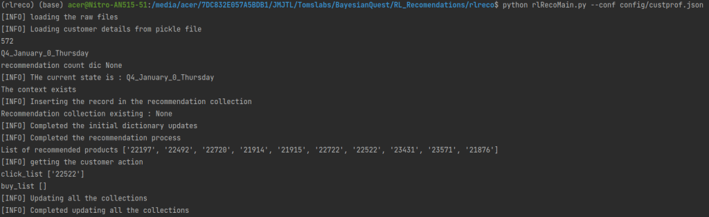
Figure 1 : Running the application on terminal
The application can be executed on the terminal with the below command
The argument we give is the path to the configuration file. Please note that we need to change directory to the rlreco directory to run this code. The output from the implementation would be as below
The data can be seen in the MongoDB collections also. Let us look at ways to find the data in MongoDB collections.
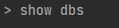
To initialise Mongo db from terminal, use the following command
Figure 3 : Initialize Mongo
You should get the following output
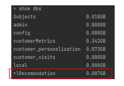
Now to find all the data bases in Mongo DB you can use the below command
You will be able to see all the databases which you have created. The one marked in red is the database we created. No to use that data base the command used is use rlRecomendation as shown below. We will get the command that the database has been switched to the desired data base.
To see all the collections we have made in this database we can use the below command.
From the output we can see all the collections we have created. Now to see some specific record within the collections, we can use the following command.
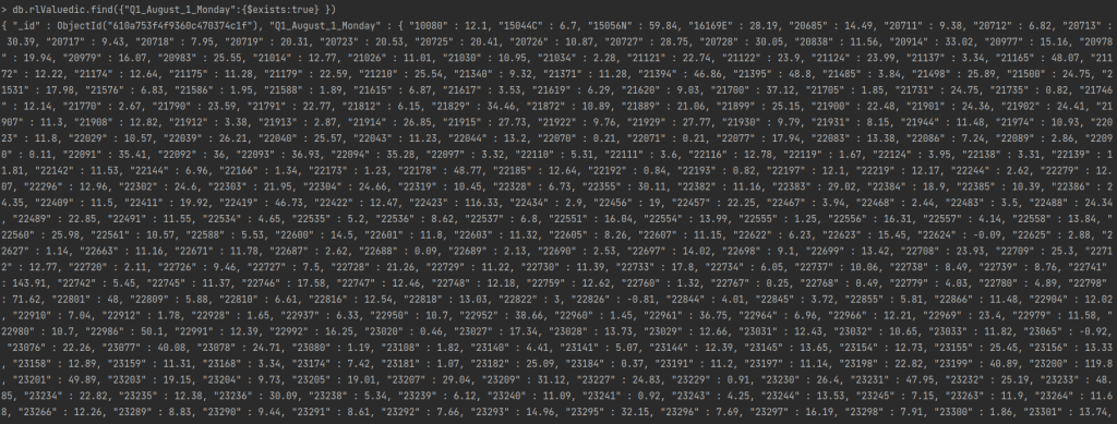
In the above command we are trying to find all records in the collection rlValuedic for the stateID "Q1_August_1_Monday". Once we execute this command we get all the records in this collection for this specific stateID. You should get the below output.
The output displays all the proucts for that stateID and its value function.
What we have implemented in code is a simulation of the complete process. To run this continuously for multiple customers, we can create another scrip with a list of desired customers and then execute the code multiple times. I will leave that step as an exercise for you to implement. Now let us look at different options to deploy this application.
Deployment of application
The end product of any data science endeavour should be to build an application and sharing it with the world. There are different options to deploy python applications. Let us look at some of the options available. I would encourage you to explore more methods and share your results.
Flask application with Heroku
A great option to deploy your applications is to package it as a Flask application and then deploy it using Heroku. We have discussed this option in one of our earlier series, where we built a machine translation application. You can refer this link for details. In this section we will discuss the nuances of building the application in Flask and then deploying it on Heroku. I will leave the implementation of the steps for you as an exercise.
When deploying the self learning recommendation system we have built, the first thing which we need to design is what the front end will contain. From the perspective of the processes we have implemented, we need to have the following processes controlled using the front end.
Training process : This is the process which takes the raw data, preprocesses the data and then initialises all the dictionaries. This includes all the processes till line 59 in the driver file rlRecoMain.py. We need to initialise the process of training from the front end of the flask application. In the background all the process till line 59 should run and the dictionaries needs to be updated.
Recommendation simulation : The second process which needs to be controlled is the one where we get the recommendations. The start of this process is the simulation of the state from the front end. To do this we can provide a drop down of all the customer IDs on the flask front end and take the system time details to form the stateID. Once this stateID is generated, we start the recommendation process which includes all the process starting from line 62 till line 90 in the the driver file rlRecoMain.py. Please note that line 64 is the stateID simulating process which will be controlled from the front end. So that line need not be implemented. The final output, which is the list of all recommended products needs to be displayed on the front end. It will be good to add some visual images along with the product for visual impact.
Customer action simulation : Once the recommended products are displayed on the front end, we can send feed back from the front end in terms of the products clicked and the products bought through some widgets created in the front end. These widgets will take the place of line 93, in our implementation. These feed back from the front end needs to be collected as lists, which will take the place of click_list and buy_list given in lines 94-95. Once the customer actions are generated, the back end process in line 98, will have to kick in to update the dictionaries. Once the cycle is completed we can build a refresh button on the screen to simulate the recommendation process again.
Once these processes are implemented using a Flask application, the application can be deployed on Heroku. This post will give you overall guide into deploying the application on Heroku.
These are broad guidelines for building the application and then deploying them. These need not be the most efficient and effective ones. I would challenge each one of you to implement much better processes for deployment. Request you to share your implementations in the comments section below.
Other options for deployment
So far we have seen one of the option to build the application using Flask and then deploy them using Heroku. There are other options too for deployment. Some of the noteable ones are the following
Flask application on Ubuntu server
Flask application on Docker
The attached link is a great resource to learn about such deployment. I would challenge all of you to deploy using any of these implementation steps and share the implementation for the community to benefit.
Wrapping up.
This is the last post of the series and we hope that this series was informative.
We will start a new series in the near future. The next series will be on a specific problem on computer vision specifically on Object detection. In the next series we will be building a ‘Road pothole detector using different object detection algorithms. This series will touch upon different methods in object detection like Image Pyramids, RCNN, Yolo, Tensorflow Object detection API etc. Watch out this space for the next series.
Please subscribe to this blog post to get notifications when the next post is published.
Do you want to Climb the Machine Learning Knowledge Pyramid ?
Knowledge acquisition is such a liberating experience. The more you invest in your knowledge enhacement, the more empowered you become. The best way to acquire knowledge is by practical application or learn by doing. If you are inspired by the prospect of being empowerd by practical knowledge in Machine learning, subscribe to our Youtube channel
I would also recommend two books I have co-authored. The first one is specialised in deep learning with practical hands on exercises and interactive video and audio aids for learning
This is the seventh post of our series on building a self learning recommendation system using reinforcement learning. This series consists of 8 posts where in we progressively build a self learning recommendation system.
Productionising the self learning recommendation system: Part II – Implementing self learning recommendation ( This Post )
Evaluating different deployment options for the self learning recommendation systems.
This post builds on the previous post where we started off with productionizing the application using python scripts. In the last post we completed the customer segmentation part. In this post we continue from where we left off and then build the self learning system using python scripts. Let us get going.
Creation of States
Let us take a quick recap of the project structure and what we covered in the last post.
In the last post we were in the early part of our main driver file rlRecoMain.py. We explored rfmMaker class in file rfmProcess.py from the processes directory. We will now explore selfLearnProcess.py file in the same directory.
Open a new file and name it selfLearnProcess.py and insert the following code
import pandas as pd
from numpy.random import normal as GaussianDistribution
from collections import OrderedDict
from collections import Counter
import operator
from random import sample
import numpy as np
from pymongo import MongoClient
client = MongoClient(port=27017)
db = client.rlRecomendation


class rlLearn:
    def __init__(self,custDetails,conf):
        # Get the date  as a seperate column
        custDetails['Date'] = custDetails['Parse_date'].apply(lambda x: x.strftime("%d"))
        # Converting date to float for easy comparison
        custDetails['Date'] = custDetails['Date'].astype('float64')
        # Get the period of month column
        custDetails['monthPeriod'] = custDetails['Date'].apply(lambda x: int(x > conf['monthPer']))
        # Aggregate the custDetails to get a distribution of rewards
        rewardFull = custDetails.groupby(['Segment', 'Month', 'monthPeriod', 'Day', conf['product_id']])[conf['prod_qnty']].agg(
            'sum').reset_index()
        # Get these data frames for all methods
        self.custDetails = custDetails
        self.conf = conf
        self.rewardFull = rewardFull
        # Defining some dictionaries for storing the values
        self.countDic = {}  # Dictionary to store the count of products
        self.polDic = {}  # Dictionary to store the value distribution
        self.rewDic = {}  # Dictionary to store the reward distribution
        self.recoCountdic = {}  # Dictionary to store the recommendation counts

    # Method to find unique values of each of the variables
    def uniqeVars(self):
        # Finding unique value for each of the variables
        segments = list(self.rewardFull.Segment.unique())
        months = list(self.rewardFull.Month.unique())
        monthPeriod = list(self.rewardFull.monthPeriod.unique())
        days = list(self.rewardFull.Day.unique())
        return segments,months,monthPeriod,days

    # Method to consolidate all products
    def prodConsolidator(self):
        # Get all the unique values of the variables
        segments, months, monthPeriod, days = self.uniqeVars()
        # Creating the consolidated dictionary
        for seg in segments:
            for mon in months:
                for period in monthPeriod:
                    for day in days:
                        # Get the subset of the data
                        subset1 = self.rewardFull[(self.rewardFull['Segment'] == seg) & (self.rewardFull['Month'] == mon) & (
                                self.rewardFull['monthPeriod'] == period) & (self.rewardFull['Day'] == day)]
                        # INitializing a temporary dictionary to storing in mongodb
                        tempDic = {}
                        # Check if the subset is valid
                        if len(subset1) > 0:
                            # Iterate through each of the subset and get the products and its quantities
                            stateId = str(seg) + '_' + mon + '_' + str(period) + '_' + day
                            # Define a dictionary for the state ID
                            self.countDic[stateId] = {}
                            tempDic[stateId] = {}
                            for i in range(len(subset1.StockCode)):
                                # Store in the Count dictionary
                                self.countDic[stateId][subset1.iloc[i]['StockCode']] = int(subset1.iloc[i]['Quantity'])
                                tempDic[stateId][subset1.iloc[i]['StockCode']] = int(subset1.iloc[i]['Quantity'])
                            # Dumping each record into mongo db
                            db.rlQuantdic.insert(tempDic)

        # Consolidate the rewards and value functions based on the quantities
        for key in self.countDic.keys():
            # Creating two temporary dictionaries for loading in Mongodb
            tempDicpol = {}
            tempDicrew = {}
            # First get the dictionary of products for a state
            prodCounts = self.countDic[key]
            self.polDic[key] = {}
            self.rewDic[key] = {}
            # Initializing temporary dictionaries also
            tempDicpol[key] = {}
            tempDicrew[key] = {}
            # Update the policy values
            for pkey in prodCounts.keys():
                # Creating the value dictionary using a Gaussian process
                self.polDic[key][pkey] = GaussianDistribution(loc=prodCounts[pkey], scale=1, size=1)[0].round(2)
                tempDicpol[key][pkey] = self.polDic[key][pkey]
                # Creating a reward dictionary using a Gaussian process
                self.rewDic[key][pkey] = GaussianDistribution(loc=prodCounts[pkey], scale=1, size=1)[0].round(2)
                tempDicrew[key][pkey] = self.rewDic[key][pkey]
            # Dumping each of these in mongo db
            db.rlRewarddic.insert(tempDicrew)
            db.rlValuedic.insert(tempDicpol)
        print('[INFO] Dumped the quantity dictionary,policy and rewards in MongoDB')
As usual we start with import of the libraries we want from lines 1-7. In this implementation we make a small deviation from the prototype which we developed in the previous post. During the prototyping phase we predominantly relied on dictionaries to store data. However here we would be storing data in Mongo DB. Those of you who are not fully conversant with MongoDB can refer to some good tutorials on MongDB like the one here. I will also be explaining the key features as and when required. In line 8, we import the MongoClient which is required for connections with the data base. We then define the client using the default port number ( 27017 ) in line 9 and then name the data base where we will store the recommendation in line 10. The name of the database we have selected is rlRecomendation . You are free to choose any name of your choice.
Let us now explore the rlLearn class. The constructor of the class which starts from line 15, takes the custDetails data frame and the configuration file as inputs. You would already be familiar with lines 17-23 from our prototyping phase, where we extract information to create states and then consolidate the data frame to get the quantities of each state. In lines 30-33, we create dictionaries where we store the relevant information like count of products, value distribution, reward distribution and the number of times the products are recommended.
The main method within the rlLearn class is the prodConslidator() method in lines 45-95. We have seen the details of this method in the prototyping phase. Just to recap, in this method we iterate through each of the components of our states and then store the quantities of each product under the state in the dictionaries. However there is a subtle difference from what we did during the prototyping phase. Here we are inserting each state and its associated products in Mongodb data base we created, as shown in line 70, 93 and 94. We create a temporary dictionary in line 57 to dump each state into Mongodb. We also store the data in the dictionaries,as we did during the prototyping phase, so that we get the data for other methods in this class. The final outcome from this method, is the creation of the count dictionary, value dictionary and reward dictionary from our data and updation of this data in Mongodb.
This takes us to the end of the rlLearn class.
We now go back to the driver file rlRecoMain.py and the explore the next important class rlRecomend.
The rlRecomend class has the methods which are required for recommending products. This class has many methods and therefore we will go one by one through each of the methods. We have seen all these methods during the prototyping phase and therefore we will not get into detailed explanation of these methods here. For detailed explanation you can refer to the previous post.
Now on the selfLearnProcess.py start adding the code pertaining to the rlRecomend class.
class rlRecomend:
    def __init__(self, custDetails, conf):
        # Get the date  as a seperate column
        custDetails['Date'] = custDetails['Parse_date'].apply(lambda x: x.strftime("%d"))
        # Converting date to float for easy comparison
        custDetails['Date'] = custDetails['Date'].astype('float64')
        # Get the period of month column
        custDetails['monthPeriod'] = custDetails['Date'].apply(lambda x: int(x > conf['monthPer']))
        # Aggregate the custDetails to get a distribution of rewards
        rewardFull = custDetails.groupby(['Segment', 'Month', 'monthPeriod', 'Day', conf['product_id']])[
            conf['prod_qnty']].agg(
            'sum').reset_index()
        # Get these data frames for all methods
        self.custDetails = custDetails
        self.conf = conf
        self.rewardFull = rewardFull
The above code is for the constructor of the class ( lines 97 – 112 ), which is similar to the constructor of the rlLearn class. Here we consolidate the custDetails data frame and get the count of each products for the respective state.
Let us now look at the next two methods. Add the following code to the class we earlier created.
# Method to find unique values of each of the variables
    def uniqeVars(self):
        # Finding unique value for each of the variables
        segments = list(self.rewardFull.Segment.unique())
        months = list(self.rewardFull.Month.unique())
        monthPeriod = list(self.rewardFull.monthPeriod.unique())
        days = list(self.rewardFull.Day.unique())
        return segments, months, monthPeriod, days

    # Method to sample a state
    def stateSample(self):
        # Get the unique state elements
        segments, months, monthPeriod, days = self.uniqeVars()
        # Get the context of the customer. For the time being let us randomly select all the states
        seg = sample(segments, 1)[0]  # Sample the segment
        mon = sample(months, 1)[0]  # Sample the month
        monthPer = sample([0, 1], 1)[0]  # sample the month period
        day = sample(days, 1)[0]  # Sample the day
        # Get the state id by combining all these samples
        stateId = str(seg) + '_' + mon + '_' + str(monthPer) + '_' + day
        self.seg = seg
        return stateId
The first method , lines 115 – 121, is to get the unique values of segments, months, month-period and days. This information will be used in some of the methods we will see later on. The second method detailed in lines 124-135, is to sample a state id, through random sampling of the components of a state.
The next methods we will explore are to initialise dictionaries if a state id has not been seen earlier. The first method initialises dictionaries and the second method inserts a recommendation collection record in MongoDB if the state dosent exist. Let us see the code for these methods.
  # Method to initialize a dictionary in case a state Id is not available
    def collfinder(self,stateId,countDic,polDic,rewDic,recoCountdic):
        # Defining some dictionaries for storing the values
        self.countDic = countDic  # Dictionary to store the count of products
        self.polDic = polDic  # Dictionary to store the value distribution
        self.rewDic = rewDic  # Dictionary to store the reward distribution
        self.recoCountdic = recoCountdic  # Dictionary to store the recommendatio
        self.stateId = stateId
        print("[INFO] The current state is :", stateId)
        if self.countDic is None:
            print("[INFO] State ID do not exist")
            self.countDic = {}
            self.countDic[stateId] = {}
            self.polDic = {}
            self.polDic[stateId] = {}
            self.rewDic = {}
            self.rewDic[stateId] = {}
        if self.recoCountdic is None:
            self.recoCountdic = {}
            self.recoCountdic[stateId] = {}
        else:
            self.recoCountdic[stateId] = {}

# Method to update the recommendation dictionary
    def recoCollChecker(self):
        print("[INFO] Inside the recommendation collection")
        recoCol = db.rlRecotrack.find_one({self.stateId: {'$exists': True}})
        if recoCol is None:
            print("[INFO] Inserting the record in the recommendation collection")
            db.rlRecotrack.insert_one({self.stateId: {}})
        return recoCol
The inputs to the first method, as in line 138 are the state Id and all the other 4 dictionaries we extract from Mongo DB, which we will see later on in the main script rlRecoMain.py. If no record exists for a specific state Id, the dictionaries we extract from Mongo DB would be null and therefore we need to initialize these dictionaries for storing all the values of products, its values, rewards and the count of recommendations. The initialisation of these dictionaries are implemented in this method from lines 146-158.
The second initialisation method is to check for the recommendation count dictionary for a specific state Id. We first check for the state Id in the collection in line 163. If the record dosent exist then we insert a blank dictionary for that state in line 166.
Let us now look at the next two methods in the class
    # Create a function to get a list of products for a certain segment
    def segProduct(self,seg, nproducts):
        # Get the list of unique products for each segment
        seg_products = list(self.rewardFull[self.rewardFull['Segment'] == seg]['StockCode'].unique())
        seg_products = sample(seg_products, nproducts)
        return seg_products

    # This is the function to get the top n products based on value
    def sortlist(self,nproducts,seg):
        # Get the top products based on the values and sort them from product with largest value to least
        topProducts = sorted(self.polDic[self.stateId].keys(), key=lambda kv: self.polDic[self.stateId][kv])[-nproducts:][::-1]
        # If the topProducts is less than the required number of products nproducts, sample the delta
        while len(topProducts) < nproducts:
            print("[INFO] top products less than required number of products")
            segProducts = self.segProduct(seg, (nproducts - len(topProducts)))
            newList = topProducts + segProducts
            # Finding unique products
            topProducts = list(OrderedDict.fromkeys(newList))
        return topProducts
The method in lines 171-175 is to sample a list of products for a segment. This method is used incase the number of products in a particular state is less than the total number of products which we want to recommend. In such cases, we randomly sample some products from the list of all products bought by customers in that segment and then add it to the list of products we want to recommend. We will see this in action in sortlist method (lines 178-188).
The sortlist method, sorts the list of products based on the demand for that product and the returns the list of top products. The inputs to this method are the number of products we want to be recommended and the segment ( line 178 ). We then get the top ‘n‘ products by sorting the value dictionary based on the number of times a product is bought as in line 180. If the number of products is less than the required products, sampling of products is done using the segProduct method we saw earlier. The final list of top products is then returned by this method.
The next method which we are going to explore is the one which controls the exploration and exploitation process thereby generating a list of products to be recommended. Let us add the following code to the class.
# This is the function to create the number of products based on exploration and exploitation
    def sampProduct(self,seg, nproducts,epsilon):
        # Initialise an empty list for storing the recommended products
        seg_products = []
        # Get the list of unique products for each segment
        Segment_products = list(self.rewardFull[self.rewardFull['Segment'] == seg]['StockCode'].unique())
        # Get the list of top n products based on value
        topProducts = self.sortlist(nproducts,seg)
        # Start a loop to get the required number of products
        while len(seg_products) < nproducts:
            # First find a probability
            probability = np.random.rand()
            if probability >= epsilon:
                # print(topProducts)
                # The top product would be first product in the list
                prod = topProducts[0]
                # Append the selected product to the list
                seg_products.append(prod)
                # Remove the top product once appended
                topProducts.pop(0)
                # Ensure that seg_products is unique
                seg_products = list(OrderedDict.fromkeys(seg_products))
            else:
                # If the probability is less than epsilon value randomly sample one product
                prod = sample(Segment_products, 1)[0]
                seg_products.append(prod)
                # Ensure that seg_products is unique
                seg_products = list(OrderedDict.fromkeys(seg_products))
        return seg_products
The inputs to the method are the segment, number of products to be recommended and the epsilon value which determines exploration and exploitation as shown in line 191. In line 195, we get the list of the products for the segment. This list is from where products are sampled during the exploration phase. We also get the list of top products which needs to be recommended in line 197, using the sortlist method we defined earlier. In lines 199-218 we implement the exploitation and exploration processes we discussed during the prototyping phase and finally we return the list of top products for recommendation.
The next method which we will explore is the one to update dictionaries after the recommendation process.
# This is the method for updating the dictionaries after recommendation
    def dicUpdater(self,prodList, stateId):
        for prod in prodList:
            # Check if the product is in the dictionary
            if prod in list(self.countDic[stateId].keys()):
                # Update the count by 1
                self.countDic[stateId][prod] += 1
            else:
                self.countDic[stateId][prod] = 1
            if prod in list(self.recoCountdic[stateId].keys()):
                # Update the recommended products with 1
                self.recoCountdic[stateId][prod] += 1
            else:
                # Initialise the recommended products as 1
                self.recoCountdic[stateId][prod] = 1
            if prod not in list(self.polDic[stateId].keys()):
                # Initialise the value as 0
                self.polDic[stateId][prod] = 0
            if prod not in list(self.rewDic[stateId].keys()):
                # Initialise the reward dictionary as 0
                self.rewDic[stateId][prod] = GaussianDistribution(loc=0, scale=1, size=1)[0].round(2)
        print("[INFO] Completed the initial dictionary updates")
The inputs to this method, as in line 221, are the list of products to be recommended and the state Id. From lines 222-234, we iterate through each of the recommended product and increament the count in the dictionary if the product exists in the dictionary or initialize the count to 1 if the product wasnt available. Later on in lines 235-240, we initialise the value dictionary and the reward dictionary if the products are not available in them.
The next method we will see is the one for initializing the dictionaries in case the context dosent exist.
    def dicAdder(self,prodList, stateId):
        # Loop through the product list
        for prod in prodList:
            # Initialise the count as 1
            self.countDic[stateId][prod] = 1
            # Initialise the value as 0
            self.polDic[stateId][prod] = 0
            # Initialise the recommended products as 1
            self.recoCountdic[stateId][prod] = 1
            # Initialise the reward dictionary as 0
            self.rewDic[stateId][prod] = GaussianDistribution(loc=0, scale=1, size=1)[0].round(2)
        print("[INFO] Completed the dictionary initialization")
        # Next update the collections with the respective updates
        # Updating the quantity collection
        db.rlQuantdic.insert_one({stateId: self.countDic[stateId]})
        # Updating the recommendation tracking collection
        db.rlRecotrack.insert_one({stateId: self.recoCount[stateId]})
        # Updating the value function collection for the products
        db.rlValuedic.insert_one({stateId: self.polDic[stateId]})
        # Updating the rewards collection
        db.rlRewarddic.insert_one({stateId: self.rewDic[stateId]})
        print('[INFO] Completed updating all the collections')
If the state Id dosent exist, the dictionaries are initialised as seen in lines 147-155. Once the dictionaries are initialised, MongoDb data bases are updated in lines 259-265.
The next method which we are going to explore is one of the main methods which integrates all the methods we have seen so far. This methods implements the recomendation process. Let us explore this method.
# Method to sample a stateID and then initialize the dictionaries
    def rlRecommender(self):
        # First sample a stateID
        stateId = self.stateId
        # Start the recommendation process
        if len(self.polDic[stateId]) > 0:
            print("The context exists")
            # Implement the sampling of products based on exploration and exploitation
            seg_products = self.sampProduct(self.seg, self.conf["nProducts"],self.conf["epsilon"])
            # Check if the recommendation count collection exist
            recoCol = self.recoCollChecker()
            print('Recommendation collection existing :',recoCol)
            # Update the dictionaries of values and rewards
            self.dicUpdater(seg_products, stateId)
        else:
            print("The context dosent exist")
            # Get the list of relavant products
            seg_products = self.segProduct(self.seg, conf["nProducts"])
            # Add products to the value dictionary and rewards dictionary
            self.dicAdder(seg_products, stateId)
        print("[INFO] Completed the recommendation process")

        return seg_products
The first step in the process is to get the state Id ( line 271 ) based on which we have to do all the recommendations. Once we have the state Id, we check if it is an existing state id in line 273. If it is an existing state Id we get the list of ‘n’ products for recommendation using the sampProduct method we saw earlier, where we implement exploration and exploitation. Once we get the products we initialise the recommendation collection in line 278. Finally we update all dictionaries using the dicUpdater method in line 281.
From lines 282-287, we implement a similar process when the state Id dosent exist. The only difference in this case is in the initialisation of the dictionaries in line 287, where we use the dicAdder method.
Once we complete the recommendation process, we get into simulating the customer action.
# Function to initiate customer action
    def custAction(self,segproducts):
        print('[INFO] getting the customer action')
        # Sample a value to get how many products will be clicked
        click_number = np.random.choice(np.arange(0, 10),
                                        p=[0.50, 0.35, 0.10, 0.025, 0.015, 0.0055, 0.002, 0.00125, 0.00124, 0.00001])
        # Sample products which will be clicked based on click number
        click_list = sample(segproducts, click_number)

        # Sample for buy values
        buy_number = np.random.choice(np.arange(0, 10),
                                      p=[0.70, 0.15, 0.10, 0.025, 0.015, 0.0055, 0.002, 0.00125, 0.00124, 0.00001])
        # Sample products which will be bought based on buy number
        buy_list = sample(segproducts, buy_number)

        return click_list, buy_list
Lines 296-305 implements the processes for simulating the list of products which are bought and browsed by the customer based on the recommendation we made. The method returns the list of products which were browsed through and also the one which were bought. For detailed explanations on these methods please refer the previous post
The next methods we will explore are the ones related to the value updation of the recommendation system.
    def getReward(self,loc):
        rew = GaussianDistribution(loc=loc, scale=1, size=1)[0].round(2)
        return rew

    def saPolicy(self,rew, prod):
        # This function gets the relavant algorithm for the policy update
        # Get the current value of the state
        vcur = self.polDic[self.stateId][prod]
        # Get the counts of the current product
        n = self.recoCountdic[self.stateId][prod]
        # Calculate the new value
        Incvcur = (1 / n) * (rew - vcur)
        return Incvcur
The getReward method on line 309 is to generate a reward from a gaussian distribution centred around the reward value. We will see the use of this method in subsequent methods.
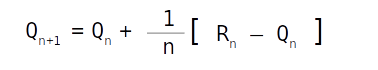
The saPolicy method in lines 313-321 updates the value of the state based on the simple averaging method in line 320. We have already seen these methods in our prototyping phase in the previous post.
Next we will see the method which uses both the above methods.
    def valueUpdater(self,seg_products, loc, custList, remove=True):
        for prod in custList:
            # Get the reward for the bought product. The reward will be centered around the defined reward for each action
            rew = self.getReward(loc)
            # Update the reward in the reward dictionary
            self.rewDic[self.stateId][prod] += rew
            # Update the policy based on the reward
            Incvcur = self.saPolicy(rew, prod)
            self.polDic[self.stateId][prod] += Incvcur
            # Remove the bought product from the product list
            if remove:
                seg_products.remove(prod)
        return seg_products
The inputs to this method are the recommended list of products, the mean reward ( click, buy or ignore), the corresponding list ( click list or buy list) and a flag to indicate if the product has to be removed from the recommendation list or not.
We interate through all the products in the customer action list in line 324 and then gets the reward in line 326. Once the reward is incremented in the reward dictionary in line 328, we get the incremental value in line 330 and this is updated in the value dictionary in line 331. If the flag is True, we remove the product from the recommended list and the finally returns the remaining recommendation list.
The next method is the last of the methods and ties the above three methods with the customer action.
# Function to update the reward dictionary and the value dictionary based on customer action
    def rewardUpdater(self, seg_products,custBuy=[], custClick=[]):
        # Check if there are any customer purchases
        if len(custBuy) > 0:
            seg_products = self.valueUpdater(seg_products, self.conf['buyReward'], custBuy)
            # Repeat the same process for customer click
        if len(custClick) > 0:
            seg_products = self.valueUpdater(seg_products, self.conf['clickReward'], custClick)
            # For those products not clicked or bought, give a penalty
        if len(seg_products) > 0:
            custList = seg_products.copy()
            seg_products = self.valueUpdater(seg_products, -2, custList,False)
        # Next update the collections with the respective updates
        print('[INFO] Updating all the collections')
        # Updating the quantity collection
        db.rlQuantdic.replace_one({self.stateId: {'$exists': True}}, {self.stateId: self.countDic[self.stateId]})
        # Updating the recommendation tracking collection
        db.rlRecotrack.replace_one({self.stateId: {'$exists': True}}, {self.stateId: self.recoCountdic[self.stateId]})
        # Updating the value function collection for the products
        db.rlValuedic.replace_one({self.stateId: {'$exists': True}}, {self.stateId: self.polDic[self.stateId]})
        # Updating the rewards collection
        db.rlRewarddic.replace_one({self.stateId: {'$exists': True}}, {self.stateId: self.rewDic[self.stateId]})
        print('[INFO] Completed updating all the collections')
In lines 340-348, we update the value based on the number of products bought, clicked and ignored. Once the value dictionaries are updated, the respective MongoDb dictionaries are updated in lines 352-358.
With this we have covered all the methods which are required for implementing the self learning recommendation system. Let us summarise our learning so far in this post.
Created the states and updated MongoDB with the states data. We used the historic data for initialisation of values.
Implemented the recommendation process by getting a list of products to be recommended to the customer
Explored customer response simulation wherein the customer response to the recommended products were implemented.
Updated the value functions and reward functions after customer response
Updated Mongo DB collections after the completion of the process for a customer.
What next ?
We are coming to the fag end of our series. The next post is where we tie all these methods together in the main driver file and see how these processes are implmented. We will also run the script on the terminal and observe the results. Once the application implementation is done, we will also explore avenues to deploy the application. Watch this space for the last post of the series.
Please subscribe to this blog post to get notifications when the next post is published.
Do you want to Climb the Machine Learning Knowledge Pyramid ?
Knowledge acquisition is such a liberating experience. The more you invest in your knowledge enhacement, the more empowered you become. The best way to acquire knowledge is by practical application or learn by doing. If you are inspired by the prospect of being empowerd by practical knowledge in Machine learning, subscribe to our Youtube channel
I would also recommend two books I have co-authored. The first one is specialised in deep learning with practical hands on exercises and interactive video and audio aids for learning
This is the sixth post of our series on building a self learning recommendation system using reinforcement learning. This series consists of 8 posts where in we progressively build a self learning recommendation system. This series consists of the following posts
Productionising the self learning recommendation system: Part I – Customer Segmentation ( This post )
Productionising the self learning recommendation system: Part II – Implementing self learning recommendation
Evaluating different deployment options for the self learning recommendation systems.
This post builds on the previous post where we started off with building the prototype of the application in Jupyter notebooks. In this post we will see how to convert our prototype into Python scripts. Converting into python script is important because that is the basis for building an application and then deploying them for general consumption.
File Structure for the project
First let us look at the file structure of our project.
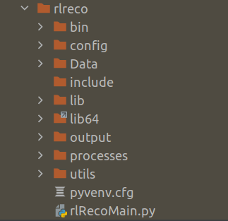
The directory RL_Recomendations is the main directory which contains other folders which are required for the project. Out of the directories rlreco is a virtual environment we will create and all our working directories are within this virtual environment.Along with the folders we also have the script rlRecoMain.py which is the main driver script for the application. We will now go through some of the steps in creating this folder structure
When building an application it is always a good practice to create a virtual environment and then complete the application build process within the virtual environment. We talked about this in one of our earlier series for building machine translation applications . This way we can ensure that only application specific libraries and packages are present when we deploy our application.
Let us first create a separate folder in our drive and then create a virtual environment within that folder. In a Linux based system, a seperate folder can be created as follows
$ mkdir RL_Recomendations
Once the new directory is created let us change directory into the RL_Recomendations directory and then create a virtual environment. A virtual environment can be created on Linux with Python3 with the below script
RL_Recomendations $ python3 -m venv rlreco
Here the rlreco is the name of our virtual environment. The virtual environment which we created can be activated as below
RL_Recomendations $ source rlreco/bin/activate
Once the virtual environment is enabled we will get the following prompt.
(rlreco) ~$
In addition you will notice that a new folder created with the same name as the virtual environment. We will use that folder to create all our folders and main files required for our application. Let us traverse through our driver file and then create all the folders and files required for our application.
Create the driver file
Open a file using your favourite editor and name it rlRecoMain.py and the insert the following code.
import argparse
import pandas as pd
from utils import Conf,helperFunctions
from Data import DataProcessor
from processes import rfmMaker,rlLearn,rlRecomend
from utils import helperFunctions
import os.path
from pymongo import MongoClient
Lines 1-2 we import the libraries which we require for our application. In line 3 we have to import Conf class from the utils folder.
So first let us create a folder called utils, which will have the following file structure.
The utils folder has a file called Conf.py which contains the Conf class and another file called helperFunctions.py . The first file controls the configuration functions and the second file contains some of the helper functions like saving data into pickle files. We will get to that in a moment.
First let us open a new python file Conf.py and copy the following code.
from json_minify import json_minify
import json

class Conf:

    def __init__(self,confPath):
        # Read the json file and load it into a dictionary
        conf = json.loads(json_minify(open(confPath).read()))
        self.__dict__.update(conf)
    def __getitem__(self, k):
        return self.__dict__.get(k,None)
The Conf class is a simple class, with its constructor loading the configuration file which is in json format in line 8. Once the configuration file is loaded the elements are extracted by invoking ‘conf’ method. We will see more of how this is used later.
We have talked about the Conf class which loads the configuration file, however we havent made the configuration file yet. As you may know a configuration file contains all the parameters in the application. Let us see the directory structure of the configuration file.
Figure : config folder and configuration file
You can now create the folder called config, under the rlreco folder and then open a file in your editor and then name it custprof.json and include the following code.
As you can see the config, file contains all the configuration items required as part of the application. The first part is where the paths to the raw file and processed pickle files are stored. The second part is the mapping of the column names in the raw file and the names used in our application. The third part contains all the parameters required for the application. The Conf class which we earlier saw will read the json file and all these parameters will be loaded to memory for us to be used in the application.
Lets come back to the utils folder and create the second file which we will name as helperFunctions.py and insert the following code.
from pickle import load
from pickle import dump
import numpy as np


# Function to Save data to pickle form
def save_clean_data(data,filename):
    dump(data,open(filename,'wb'))
    print('Saved: %s' % filename)

# Function to load pickle data from disk
def load_files(filename):
    return load(open(filename,'rb'))
This file contains two functions. The first function starting in line 7 saves a file in pickle format to the specified path. The second function in line 12, loads a pickle file and return the data. These two functions are handy functions which will be used later in our project.
We will come back to the main file rlRecoMain.py and look at the next folder and methods on line 4. In this line we import DataProcessor method from the folder Data . Let us take a look at the folder called Data.
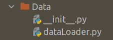
Create the data processor module
The class and the methods associated with the class are in the file dataLoader.py. Let us first create the folder, Data and then open a file named dataLoader.py and insert the following code.
import os
import pandas as pd
import pickle
import numpy as np
import random
from utils import helperFunctions
from datetime import datetime, timedelta,date
from dateutil.parser import parse
class DataProcessor:
def __init__(self,configfile):
# This is the first method in the DataProcessor class
self.config = configfile
# This is the method to load data from the input files
def dataLoader(self):
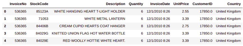
inputPath = self.config["inputData"]
dataFrame = pd.read_csv(inputPath,encoding = "ISO-8859-1")
return dataFrame
# This is the method for parsing dates
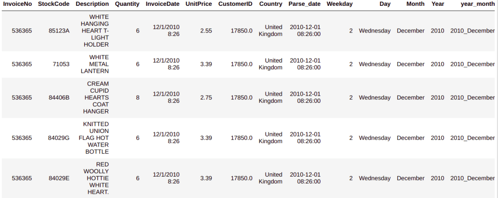
def dateParser(self):
custDetails = self.dataLoader()
#Parsing the date
custDetails['Parse_date'] = custDetails[self.config["order_date"]].apply(lambda x: parse(x))
# Parsing the weekdaty
custDetails['Weekday'] = custDetails['Parse_date'].apply(lambda x: x.weekday())
# Parsing the Day
custDetails['Day'] = custDetails['Parse_date'].apply(lambda x: x.strftime("%A"))
# Parsing the Month
custDetails['Month'] = custDetails['Parse_date'].apply(lambda x: x.strftime("%B"))
# Getting the year
custDetails['Year'] = custDetails['Parse_date'].apply(lambda x: x.strftime("%Y"))
# Getting year and month together as one feature
custDetails['year_month'] = custDetails['Year'] + "_" +custDetails['Month']
return custDetails
def gvCreator(self):
custDetails = self.dateParser()
# Creating gross value column
custDetails['grossValue'] = custDetails[self.config["prod_qnty"]] * custDetails[self.config["unit_price"]]
return custDetails
The constructor of the DataProcessor class takes the config file as the input and then make it available for all the other methods in line 13.
This dataProcessor class will have three methods, dataLoader, dateParser and gvCreator. The last method is the driving method which internally calls other two methods. Let us look at the gvCreator method.
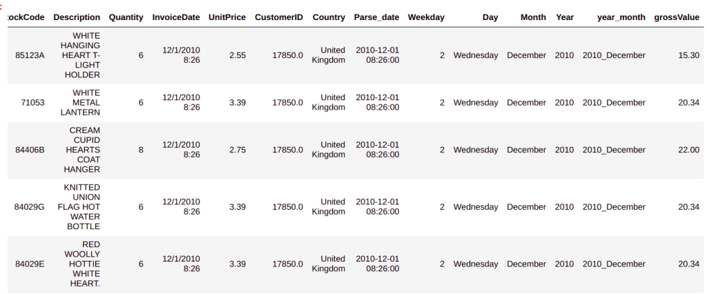
The dateParser method is called first within the gvCreator method in line 40. The dateParser method in turn calls the dataLoader method in line 23. The dataLoader method loads the customer data as a pandas data frame in line 18 and the passes it to the dateParser method in line 23. The dateParser method takes the custDetails data frame and then extracts all the date related fields from lines 25-35. We saw this in detail during the prototyping phase in the previous post.
Once the dates are parsed in the custDetails data frame, it is passed to gvCreator method in line 40 and then the ‘gross value’ is calcuated by multiplying the unit price and the product quantity. Finally the processed custDetails file is returned.
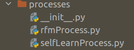
Now we will come back to the rlRecoMain file and the look at the three other classes, rfmMaker,rlLearn,rlRecomend, we import in line 5 of the file rlRecoMain.py. This is imported from the ‘processes’ folder. Let us look at the composition of the processes folder.
We have three files in the folder, processes.
The first one is the __init__.py file which is the constructor to the package. Let us see its contentes. Open a file and name it __init__.py and add the following lines of code.
from .rfmProcess import rfmMaker
from .selfLearnProcess import rlLearn,rlRecomend
Create customer segmentation modules
In lines 1-2 of the constructor file we make the three classes ( rfmMaker,rlLearn and rlRecomend) available to the package. The class rfmMaker is in the file rfmProcess.py and the other two classes are in the file selfLearnProcess.py.
Let us open a new file, name it rfmProcess.py and then insert the following code.
import sys
sys.path.append('path_to_the_folder/RL_Recomendations/rlreco')
import pandas as pd
import lifetimes
from sklearn.cluster import KMeans
from utils import helperFunctions
class rfmMaker:
def __init__(self,custDetails,conf):
self.custDetails = custDetails
self.conf = conf
def rfmMatrix(self):
# Converting data to RFM format
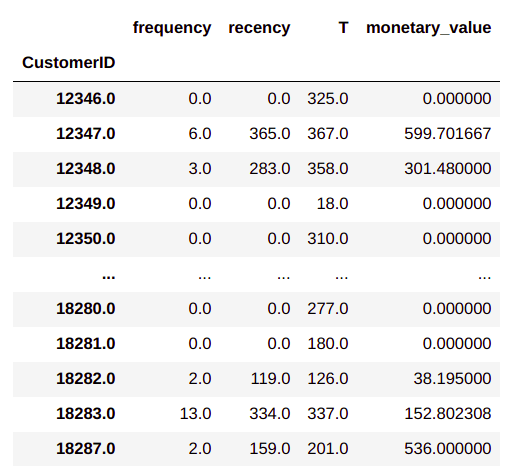
RfmAgeTrain = lifetimes.utils.summary_data_from_transaction_data(self.custDetails, self.conf['customer_id'], 'Parse_date','grossValue')
# Reset the index
RfmAgeTrain = RfmAgeTrain.reset_index()
return RfmAgeTrain
# Function for ordering cluster numbers
def order_cluster(self,cluster_field_name, target_field_name, data, ascending):
# Group the data on the clusters and summarise the target field(recency/frequency/monetary) based on the mean value
data_new = data.groupby(cluster_field_name)[target_field_name].mean().reset_index()
# Sort the data based on the values of the target field
data_new = data_new.sort_values(by=target_field_name, ascending=ascending).reset_index(drop=True)
# Create a new column called index for storing the sorted index values
data_new['index'] = data_new.index
# Merge the summarised data onto the original data set so that the index is mapped to the cluster
data_final = pd.merge(data, data_new[[cluster_field_name, 'index']], on=cluster_field_name)
# From the final data drop the cluster name as the index is the new cluster
data_final = data_final.drop([cluster_field_name], axis=1)
# Rename the index column to cluster name
data_final = data_final.rename(columns={'index': cluster_field_name})
return data_final
# Function to do the cluster ordering for each cluster
#
def clusterSorter(self,target_field_name,RfmAgeTrain, ascending):
# Defining the number of clusters
nclust = self.conf['nclust']
# Make the subset data frame using the required feature
user_variable = RfmAgeTrain[['CustomerID', target_field_name]]
# let us take four clusters indicating 4 quadrants
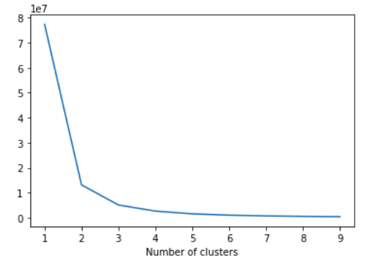
kmeans = KMeans(n_clusters=nclust)
kmeans.fit(user_variable[[target_field_name]])
# Create the cluster field name from the target field name
cluster_field_name = target_field_name + 'Cluster'
# Create the clusters
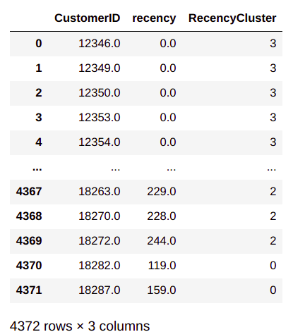
user_variable[cluster_field_name] = kmeans.predict(user_variable[[target_field_name]])
# Sort and reset index
user_variable.sort_values(by=target_field_name, ascending=ascending).reset_index(drop=True)
# Sort the data frame according to cluster values
user_variable = self.order_cluster(cluster_field_name, target_field_name, user_variable, ascending)
return user_variable
def clusterCreator(self):
#data : THis is the dataframe for which we want to create the clsuters
#clustName : This is the variable name
#nclust ; Numvber of clusters to be created
# Get the RFM data Frame
RfmAgeTrain = self.rfmMatrix()
# Implementing for user recency
user_recency = self.clusterSorter('recency', RfmAgeTrain,False)
#print('recency grouping',user_recency.groupby('recencyCluster')['recency'].mean().reset_index())
# Implementing for user frequency
user_freqency = self.clusterSorter('frequency', RfmAgeTrain, True)
#print('frequency grouping',user_freqency.groupby('frequencyCluster')['frequency'].mean().reset_index())
# Implementing for monetary values
user_monetary = self.clusterSorter('monetary_value', RfmAgeTrain, True)
#print('monetary grouping',user_monetary.groupby('monetary_valueCluster')['monetary_value'].mean().reset_index())
# Merging the individual data frames with the main data frame
RfmAgeTrain = pd.merge(RfmAgeTrain, user_monetary[["CustomerID", 'monetary_valueCluster']], on='CustomerID')
RfmAgeTrain = pd.merge(RfmAgeTrain, user_freqency[["CustomerID", 'frequencyCluster']], on='CustomerID')
RfmAgeTrain = pd.merge(RfmAgeTrain, user_recency[["CustomerID", 'recencyCluster']], on='CustomerID')
# Calculate the overall score
RfmAgeTrain['OverallScore'] = RfmAgeTrain['recencyCluster'] + RfmAgeTrain['frequencyCluster'] + RfmAgeTrain['monetary_valueCluster']
return RfmAgeTrain
def segmenter(self):
#This is the script to create segments after the RFM analysis
# Get the RFM data Frame
RfmAgeTrain = self.clusterCreator()
# Segment data
RfmAgeTrain['Segment'] = 'Q1'
RfmAgeTrain.loc[(RfmAgeTrain.OverallScore == 0), 'Segment'] = 'Q2'
RfmAgeTrain.loc[(RfmAgeTrain.OverallScore == 1), 'Segment'] = 'Q2'
RfmAgeTrain.loc[(RfmAgeTrain.OverallScore == 2), 'Segment'] = 'Q3'
RfmAgeTrain.loc[(RfmAgeTrain.OverallScore == 4), 'Segment'] = 'Q4'
RfmAgeTrain.loc[(RfmAgeTrain.OverallScore == 5), 'Segment'] = 'Q4'
RfmAgeTrain.loc[(RfmAgeTrain.OverallScore == 6), 'Segment'] = 'Q4'
# Merging the customer details with the segment
custDetails = pd.merge(self.custDetails, RfmAgeTrain, on=['CustomerID'], how='left')
# Saving the details as a pickle file
helperFunctions.save_clean_data(custDetails,self.conf["custDetails"])
print("[INFO] Saved customer details ")
return custDetails
The rfmMaker, class contains methods which does the following tasks,Converting the custDetails data frame to the RFM format. We saw this method in the previous post, where we used the lifetimes library to convert the data frame to the RFM format. This process is detailed in the rfmMatrix method from lines 15-20.
Once the data is made in the RFM format, the next task as we saw in the previous post was to create the clusters for recency, frequency and monetary values. During our prototyping phase we decided to adopt 4 clusters for each of these variables. In this method we will pass the number of clusters through the configuration file as seen in line 44 and then we create these clusters using Kmeans method as shown in lines 48-49. Once the clusters are created, the clusters are sorted to get a logical order. We saw these steps during the prototyping phase and these are implemented using clusterCreator method ( lines 61-85)clusterSorter method ( lines 42-58 ) and orderCluster methods ( lines 24 – 37 ). As the name suggests the first method is to create the cluster and the latter two are to sort it in the logical way. The detailed explanations of these functions are detailed in the last post.
After the clusters are made and sorted, the next task was to merge it with the original data frame. This is done in the latter part of the clusterCreator method ( lines 80-82 ). As we saw in the prototyping phase we merged all the three cluster details to the original data frame and then created the overall score by summing up the scores of each of the individual clusters ( line 84 ) . Finally this data frame is returned to the final method segmenter for defining the segments
Our final task was to combine the clusters to 4 distinct segments as seen from the protoyping phase. We do these steps in the segmenter method ( lines 94-100 ). After these steps we have 4 segments ‘Q1’ to ‘Q4’ and these segments are merged to the custDetails data frame ( line 103 ).
Thats takes us to the end of this post. So let us summarise all our learning so far in this post.
Created the folder structure for the project
Created a virtual environment and activated the virtual environment
Created folders like Config, Data, Processes, Utils and the created the corresponding files
Created the code and files for data loading, data clustering and segmenting using the RFM process
We will not get into other aspects of building our self learning system in the next post.
What Next ?
Now that we have explored rfmMaker class in file rfmProcess.pyin the next post we will define the classes and methods for implementing the recommendation and self learning processes. The next post will be published next week. To be notified of the next post please subscribe to this blog post .You can also subscribe to our Youtube channel for all the videos related to this series.
Do you want to Climb the Machine Learning Knowledge Pyramid ?
Knowledge acquisition is such a liberating experience. The more you invest in your knowledge enhacement, the more empowered you become. The best way to acquire knowledge is by practical application or learn by doing. If you are inspired by the prospect of being empowerd by practical knowledge in Machine learning, subscribe to our Youtube channel
I would also recommend two books I have co-authored. The first one is specialised in deep learning with practical hands on exercises and interactive video and audio aids for learning
This is the fifth post of our series on building a self learning recommendation system using reinforcement learning. This post of the series builds on the previous post where we segmented customers using RFM analysis. This series consists of the following posts.
Build the prototype of the self learning recommendation system: Part II ( This post )
Productionising the self learning recommendation system: Part I – Customer Segmentation
Productionising the self learning recommendation system: Part II – Implementing self learning recommendation
Evaluating different deployment options for the self learning recommendation systems.
Introduction
In the last post we saw how to create customer segments from transaction data. In this post we will use the customer segments to create states of the customer. Before making the states let us make some assumptions based on the buying behaviour of customers.
Customers in the same segment have very similar buying behaviours
The second assumption we will make is that buying pattern of customers vary accross the months. Within each month we are assuming that the buying behaviour within the first 15 days is different from the buying behaviour in the next 15 days. Now these assumptions are made only to demonstrate how such assumptions will influence the creation of different states of the customer. One can still go much more granular with assumptions that the buying pattern changes every week in a month, i.e say the buying pattern within the first week will be differnt from that of the second week and so on. With each level of granularity the number of states required will increase. Ideally such decisions need to be made considering the business dynamics and based on real customer buying behaviours.
The next assumption we will be making is based on the days in a week. We make an assumption that buying behaviours of customers during different days of a week also varies.
Based on these assumptions, each state will have four tiers i.e
Customer segment >> month >> within first 15 days or not >> day of the week.
Let us now see how this assumption can be carried forward to create different states for our self learning recommendation system.
As a first step towards creation of states, we will create some more variables from the existing variables. We will be using the same dataframe we created till the segmentation phase, which we discussed in the last post.
# Feature engineering of the customer details data frame
# Get the date  as a seperate column
custDetails['Date'] = custDetails['Parse_date'].apply(lambda x: x.strftime("%d"))
# Converting date to float for easy comparison
custDetails['Date']  = custDetails['Date'] .astype('float64')
# Get the period of month column
custDetails['monthPeriod'] = custDetails['Date'].apply(lambda x: int(x > 15))

custDetails.head()
Let us closely look at the changes incorporated. In line 3, we are extracting the date of the month and then converting them into a float type in line 5. The purpose of taking the date is to find out which of these transactions have happened before 15th of the month and which after 15th. We extract those details in line 7, where we create a binary points ( 0 & 1) as to whether a date falls in the last 15 days or the first 15 days of the month. Now all data points required to create the state is in place. These individual data points will be combined together to form the state ( i.e. Segment-Month-Monthperiod-Day ). We will getinto nuances of state creation next.
Initialization of values
When we discussed about the K armed bandit in post 2, we saw the functions for generating the rewards and value. What we will do next is to initialize the reward function and the value function for the states.A widely used method for finding the value function and the reward function is to intialize those values to zero. However we already have data on each state and the product buying frequency for each of these states. We will aggregate the quantities of each product as per the state combination to create our initial value functions.
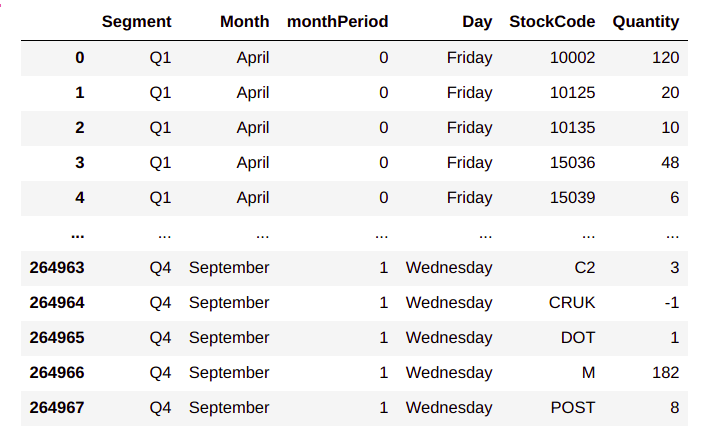
# Aggregate custDetails to get a distribution of rewards
rewardFull = custDetails.groupby(['Segment','Month','monthPeriod','Day','StockCode'])['Quantity'].agg('sum').reset_index()

rewardFull
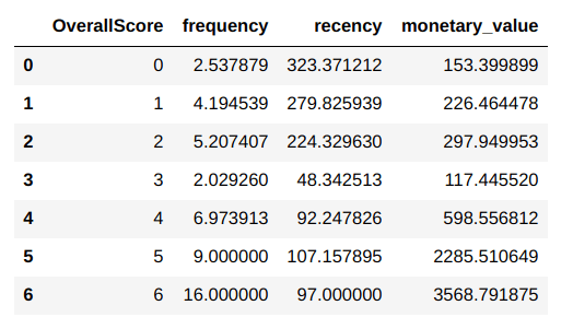
From the output, we can see the state wise distribution of products . For example for the state Q1_April_0_Friday we find that the 120 quantities of product ‘10002’ was bought and so on. So the consolidated data frame represents the propensity of buying of each product. We will make the propensity of buying the basis for the initial values of each product.
Now that we have consolidated the data, we will get into the task of creating our reward and value distribution. We will extract information relevant for each state and then load the data into different dictionaries for ease of use. We will kick off these processes by first extracting the unique values of each of the components of our states.
# Finding unique value for each of the segment
segments = list(rewardFull.Segment.unique())
print('segments',segments)
months = list(rewardFull.Month.unique())
print('months',months)
monthPeriod = list(rewardFull.monthPeriod.unique())
print('monthPeriod',monthPeriod)
days = list(rewardFull.Day.unique())
print('days',days)
In lines 16-22, we take the unique values of each of the components of our state and then store them as list. We will use these lists to create our reward an value function dictionaries . First let us create dictionaries in which we are going to store the values.
# Defining some dictionaries for storing the values
countDic = {} # Dictionary to store the count of products
polDic = {} # Dictionary to store the value distribution
rewDic = {} # Dictionary to store the reward distribution
recoCount = {} # Dictionary to store the recommendation counts
Let us now implement the process of initializing the reward and value functions.
for seg in segments:
    for mon in months:
        for period in monthPeriod:
            for day in days:
                # Get the subset of the data
                subset1 = rewardFull[(rewardFull['Segment'] == seg) & (rewardFull['Month'] == mon) & (
                            rewardFull['monthPeriod'] == period) & (rewardFull['Day'] == day)]
                # Check if the subset is valid
                if len(subset1) > 0:
                    # Iterate through each of the subset and get the products and its quantities
                    stateId = str(seg) + '_' + mon + '_' + str(period) + '_' + day
                    # Define a dictionary for the state ID
                    countDic[stateId] = {}
                    for i in range(len(subset1.StockCode)):
                        countDic[stateId][subset1.iloc[i]['StockCode']] = int(subset1.iloc[i]['Quantity'])
Thats an ugly looking loop. Let us unravel it. In lines 30-33, we implement iterative loops to go through each component of our state, starting from segment, month, month period and finally days. We then get the data which corresponds to each of the components of the state in line 35. In line 38 we do a check to see if there is any data pertaining to the state we are interested in. If there is valid data, then we first define an ID for the state, by combining all the components in line 40. In line 42, we define an inner dictionary for each element of the countDic, dictionary. The key of the countDic dictionary is the state Id we defined in line 40. In the inner dictionary we store each of the products as its key and the corresponding quantity values of the product as its values in line 44.
Let us look at the total number of states in the countDic
len(countDic)
You will notice that there are 572 states formed. Let us look at the data for some of the states.
From the output we can see how for each state, the products and its frequency of purchase is listed. This will form the basis of our reward distribution and also the value distribution. We will create that next
Consolidation of rewards and value distribution
from numpy.random import normal as GaussianDistribution
# Consolidate the rewards and value functions based on the quantities
for key in countDic.keys():
    # First get the dictionary of products for a state
    prodCounts = countDic[key]
    polDic[key] = {}
    rewDic[key] = {}
    # Update the policy values
    for pkey in prodCounts.keys():
        # Creating the value dictionary using a Gaussian process
        polDic[key][pkey] = GaussianDistribution(loc=prodCounts[pkey], scale=1, size=1)[0].round(2)
        # Creating a reward dictionary using a Gaussian process
        rewDic[key][pkey] = GaussianDistribution(loc=prodCounts[pkey], scale=1, size=1)[0].round(2)
In line 50, we iterate through each of the states in the countDic. Please note that the key of the dictionary is the state. In line 52, we store the products and its counts for a state, in another variable prodCounts. The prodCounts dictionary has the the product id as its key and the buying frequency as the value,. Lines 53 and 54, we create two more dictionaries for the value and reward dictionaries. In line 56 we loop through each product of the state and make it the key of the inner dictionaries of reward and value dictionaries. We generate a random number from a Gaussian distribution with the mean as the frequency of purchase for the product . We store the number generated from the Gaussian distribution as values for both rewards and value function dictionaries. At the end of the iterations, we get a distribution of rewards and value for each state and the products within each state. The distribution would be centred around the frequency of purchase of each of the product under the state.
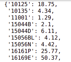
Let us take a look at some sample values of both the dictionaries
polDic[stateId]
rewDic[stateId]
We have the necessary ingradients for building our selflearning recommendation engine. Let us now think about the actual process in an online recommendation system. In the actual process when a customer visits the ecommerce site, we first need to understand the state of that customer which will be the segment of the customer, the currrent month, which half of the month the customer is logging in and also the day when the customer is logging in. These are the information we would require to create the states.
For our purpose we will simulate the context of the customer using random sampling
Simulation of customer action
# Get the context of the customer. For the time being let us randomly select all the states
seg = sample(['Q1','Q2','Q3','Q4'],1)[0] # Sample the segment
mon = sample(['January','February','March','April','May','June','July','August','September','October','November','December'],1)[0] # Sample the month
monthPer = sample([0,1],1)[0] # sample the month period
day = sample(['Sunday','Monday','Tuesday','Wednesday','Thursday','Friday','Saturday'],1)[0] # Sample the day
# Get the state id by combining all these samples
stateId = str(seg) + '_' +  mon + '_' + str(monthPer) + '_' + day
print(stateId)
Lines 64-67, we sample each component of the state and then in line 68 we combine them to form the state id. We will be using the state id for the recommendation process. The recommendation process will have the following step.
Process 1 : Initialize dictionaries
A check is done to find if the value of reward dictionares which we earlier defined has the states which we sampled. If the state exists we take the value dictionary corresponding to the sampled state, if the state dosent exist, we initialise an empty dictionary corresponding to the state. Let us look at the function to do that.
def collfinder(dictionary,stateId):
    # dictionary ; This is the dictionary where we check if the state exists
    # stateId : StateId to be checked
    if stateId in dictionary.keys():
        mycol = {}
        mycol[stateId] = dictionary[stateId]
    else:
        # Initialise the state Id in the dictionary
        dictionary[stateId] = {}
        # Return the state specific collection
        mycol = {}
        mycol[stateId] = dictionary[stateId]

    return mycol[stateId],mycol,dictionary
In line 71, we define the function. The inputs are the dictionary the state id we want to verify. We first check if the state id exists in the dictionary in line 74. If it exists we create a new dictionary called mycol in line 75 and then load all the products and its count to mycol dictionary in line 76.
If the state dosent exist, we first initialise the state in line 79 and then repeat the same processes as of lines 75-76.
Let us now implement this step for the dictionaries which we have already created.
# Check for the policy Dictionary
mypolDic,mypol,polDic = collfinder(polDic,stateId)
Let us check the mypol dictionary.
mypol
We can see the policy dictionary for the state we defined. We will now repeat the process for the reward dictionary and the count dictionaries
# Check for the Reward Dictionary
myrewDic, staterew,rewDic = collfinder(rewDic,stateId)
# Check for the Count Dictionary
myCount,quantityDic,countDic = collfinder(countDic,stateId)
Both these dictionaries are similar to the policy dictionary above.
We also will be creating a similar dictionary for the recommended products, to keep count of all the products which are recommended. Since we havent created a recommendation dictionary, we will initialise that and create the state for the recommendation dictionary.
# Initializing the recommendation dictionary
recoCountdic = {}
# Check the recommendation count dictionary
myrecoDic,recoCount,recoCountdic = collfinder(recoCountdic,stateId)
We will now get into the second process which is the recommendation process
Process 2 : Recommendation process
We start the recommendation process based on the epsilon greedy method. Let us define the overall process for the recommendation system.
As mentioned earlier, one of our basic premise was that customers within the same segment have similar buying propensities. So the products which we need to recommend for a customer, will be picked from all the products bought by customers belonging to that segment. So the first task in the process is to get all the products relevant for the segment to which the customer belongs. We sort the products, in descending order, based on the frequency of product purchase.
Implementing the self learning recommendation system using epsilon greedy process
Next we start the epsion greedy process as learned in post 2, to select the top n products we want to recommend. To begin this process, we generate a random probability distribution value. If the random value is greater than the epsilon value, we pick the first product in the sorted list of products for the segment. Once a product is picked we remove it from the list of products from the segment to ensure that we dont pick it again. This process as we learned when we implemented K-armed bandit problem, is the exploitation phase.
The above was a case when the random probability number was greater than the epsilon value, now if the random probability number is less than the epsilon value, we get into the exploration phase. We randomly sample a product from the universe of products for the segment. Here again we restrict our exploration to the universe of products relevant for the segment. However one could design the exploration ourside the universe of the segment and maybe explore from the basket of all products for all customers.
We continue the exploitation and exploration process till we get the top n products we want. We will look at some of the functions which implements this process.
# Create a function to get a list of products for a certain segment
def segProduct(seg, nproducts,rewardFull):
    # Get the list of unique products for each segment
    seg_products = list(rewardFull[rewardFull['Segment'] == seg]['StockCode'].unique())
    seg_products = sample(seg_products, nproducts)
    return seg_products

# This is the function to get the top n products based on value
def sortlist(nproducts, stateId,seg,mypol):
    # Get the top products based on the values and sort them from product with largest value to least
    topProducts = sorted(mypol[stateId].keys(), key=lambda kv: mypol[stateId][kv])[-nproducts:][::-1]
    # If the topProducts is less than the required number of products nproducts, sample the delta
    while len(topProducts) < nproducts:
        print("[INFO] top products less than required number of products")
        segProducts = segProduct(seg,(nproducts - len(topProducts)))
        newList = topProducts + segProducts
        # Finding unique products
        topProducts = list(OrderedDict.fromkeys(newList))
    return topProducts

# This is the function to create the number of products based on exploration and exploitation
def sampProduct(seg, nproducts, stateId, epsilon,mypol):
    # Initialise an empty list for storing the recommended products
    seg_products = []
    # Get the list of unique products for each segment
    Segment_products = list(rewardFull[rewardFull['Segment'] == seg]['StockCode'].unique())
    # Get the list of top n products based on value
    topProducts = sortlist(nproducts, stateId,seg,mypol)
    # Start a loop to get the required number of products
    while len(seg_products) < nproducts:
        # First find a probability
        probability = np.random.rand()
        if probability >= epsilon:
            # The top product would be first product in the list
            prod = topProducts[0]
            # Append the selected product to the list
            seg_products.append(prod)
            # Remove the top product once appended
            topProducts.pop(0)
            # Ensure that seg_products is unique
            seg_products = list(OrderedDict.fromkeys(seg_products))
        else:
            # If the probability is less than epsilon value randomly sample one product
            prod = sample(Segment_products, 1)[0]
            seg_products.append(prod)
            # Ensure that seg_products is unique
            seg_products = list(OrderedDict.fromkeys(seg_products))
    return seg_products
In line 117 we define the function to get the recommended products. The input parameters for the function are the segment, number of products we want to recommend, state id,epsilon value and the policy dictionary . We initialise a list to store the recommended products in line 119 and then extract all the products relevant for the segment in line 121. We then sort the segment products according to frequency of the products. We use the function ‘sortlist‘ in line 104 for this purpose. We sort the value dictionary according to the frequency and then select the top n products in the descending order in line 106. Now if the number of products in the dictionary is less than the number of products we want to be recommended, we randomly select the remaining products from the list of products for the segment. Lines 99-100 in the function ‘segproducts‘ is where we take the list of unique products for the segment and then randomly sample the required number of products and return it in line 110. In line 111 the additional products along with the top products is joined together. The new list of top products are sorted as per the order in which the products were added in line 112 and returned to the calling function in line 123.
Lines 125-142 implements the epsilon greedy process for product recommendation. This is a loop which continues till we get the required number of products for recommending. In line 127 a random probability score is generated and is verified whether it is greater than the epsilon value in line 128. If the random probability score is greater than epsilon value, we extract the topmost product from the list of products in line 130 and then append it to the recommendation candidate product list in line 132. After extraction of the top product, it is removed from the list in line 134. The list is sorted according to the order in which products are added in line 136. This loop continues till we get the required number of products for recommendation.
Lines 137-142 is the loop when the random score is less than the epsilon value i.e exploration stage. In this stage we randomly sample products from the list of products appealing to the segment and append it to the list of recommendation candidates. The final list of candiate products to be recommended is returned in line 143.
Process 3 : Updation of all relevant dictionaries
In the last section we saw the process of selecting the products for recommendation. The next process we will cover is how the products recommended are updated in the relevant dictionaries like quantity dictionary, value dictionary, reward dictionary and recommendation dictionary. Again we will use a function to update the dictionaries. The first function we will see is the one used to update sampled products.
def dicUpdater(prodList, stateId,countDic,recoCountdic,polDic,rewDic):
    # Loop through each of the products
    for prod in prodList:
        # Check if the product is in the dictionary
        if prod in list(countDic[stateId].keys()):
            # Update the count by 1
            countDic[stateId][prod] += 1
        else:
            countDic[stateId][prod] = 1
        if prod in list(recoCountdic[stateId].keys()):
            # Update the recommended products with 1
            recoCountdic[stateId][prod] += 1
        else:
            # Initialise the recommended products as 1
            recoCountdic[stateId][prod] = 1
        if prod not in list(polDic[stateId].keys()):
            # Initialise the value as 0
            polDic[stateId][prod] = 0
        if prod not in list(rewDic[stateId].keys()):
            # Initialise the reward dictionary as 0
            rewDic[stateId][prod] = GaussianDistribution(loc=0, scale=1, size=1)[0].round(2)

    # Return all the dictionaries after update
    return countDic,recoCountdic,polDic,rewDic
The inputs for the function are the recommended products ,prodList , stateID, count dictionary, recommendation dictionary, value dictionary and reward dictionary as shown in line 144.
A inner loop is executed in lines 146-166, to go through each product in the product list. In line 148 a check is made to find out if the product is in the count dictionary. This entails, understanding if the product was ever bought under that state. If the product was ever bought before, the count is updated by 1. However if the product was not bought earlier, then the dictionary for that product under that state is initialised as 1 in line 152.
The next step is for updating the recommendation count for the same product. The same logic as above applies. If the product was recommended before, for that state, the number is updated by 1 if not the number is initialised to 1 in lines 153-158.
The next task is to verify if there is a value distribution for this product for the specific state as in lines 159-161. If the value distribution does not exist, it is initialised to zero. However we dont do any updation to the value distribution here. The updation to value distribution happens later on. We will come to that in a moment
The last check is to verify if the product exists in the reward dictionary for that state in lines 162-164. If it dosent exist then it is initialised with a gaussian distribution. Again we dont do any updation for reward as this is done later on.
Now that we have seen the function for updating the dictionaries, we will get into a function which initializes dictionaries. This process is required, if a particular state has never been seen for any of the dictionaries. Let us get to that function
def dicAdder(prodList, stateId,countDic,recoCountdic,polDic,rewDic):
    countDic[stateId] = {}
    polDic[stateId] = {}
    recoCountdic[stateId] = {}
    rewDic[stateId] = {}
    # Loop through the product list
    for prod in prodList:
        # Initialise the count as 1
        countDic[stateId][prod] = 1
        # Initialise the value as 0
        polDic[stateId][prod] = 0
        # Initialise the recommended products as 1
        recoCountdic[stateId][prod] = 1
        # Initialise the reward dictionary as 0
        rewDic[stateId][prod] = GaussianDistribution(loc=0, scale=1, size=1)[0].round(2)
    # Return all the dictionaries after update
    return countDic,recoCountdic,polDic,rewDic
The inputs to this function as seen in line 168 are the same as what we saw in the update function. In lines 169-172, we initialise the innner dictionaries for the current state. Lines 174-182, all the inner dictionaries are initialised for the respective products. The count and recommendation dictionaries are initialised by 1 and the value dictionary is intialised as 0. The reward dictionary is initialised using a gaussian distribution. Finally the updated dictionaries are returned in line 184.
Next we start the recommendation process using all the functions we have defined so far.
nProducts = 10
epsilon=0.1

# Get the list of recommended products and update the dictionaries.The process is executed for a scenario when the context exists and does not exist
if len(mypolDic) > 0:
    print("The context exists")
    # Implement the sampling of products based on exploration and exploitation
    seg_products = sampProduct(seg, nProducts , stateId, epsilon,mypol)
    # Update the dictionaries of values and rewards
    countDic,recoCountdic,polDic,rewDic = dicUpdater(seg_products, stateId,countDic,recoCountdic,polDic,rewDic)
else:
    print("The context dosent exist")
    # Get the list of relavant products
    seg_products = segProduct(seg, nProducts)
    # Add products to the value dictionary and rewards dictionary
    countDic,recoCountdic,polDic,rewDic = dicAdder(seg_products, stateId,countDic,recoCountdic,polDic,rewDic)
We define the number of products and epsilon values in lines 185-186. In line 189 we check if the state exists which would mean that there would be some products in the dictionary. If the state exists, then we get the list of recommended products using the ‘sampProducts‘ function we saw earlier in line192. After getting the list of products we update all the dictionaries in line 194.
If the state dosent exist, then products are randomly sampled using the ‘segProduct‘ function in line198. As before we update the dictionaries in line 200.
Process 4 : Customer Action
So far we have implemented the recommendation process. In real world application, the products we generated are displayed as recommendations to the customer. Based on the recommendations received, the customer carries out different actions as below.
Customer could buy one or more of the recommended products
Customer could browse through the recommended products
Customer could ignore all the recommendations.
Based on the customer actions, we need to give feed back to the online learning system as to how good the recommendations were. Obviously the first scenario is the most desired one, the second one indicates some level of interest and the last one is the undesirable effect. From an self learning perspective we need to reinforce the desirable behaviours and discourage undesirable behavrious by devising proper rewards systems.
Just like we simulated customer states, we will create some functions to simulate customer actions. We define probability distribution to simulate customers propensity for buying a product or clicking a product. Based on the probability distribution we get how many products get bought or how many get clicked. Based on these numbers we sample products from our recommended list as to how many of them are going to be bought or how many would be clicked. Please note that these processes are only required as we are not implementing on a real system. When we are implementing this process in a real system, we get all these feedbacks from the the choices made by the customer.
def custAction(segproducts):
    print('[INFO] getting the customer action')
    # Sample a value to get how many products will be clicked
    click_number = np.random.choice(np.arange(0, 10), p=[0.50,0.35,0.10, 0.025, 0.015,0.0055, 0.002,0.00125,0.00124,0.00001])
    # Sample products which will be clicked based on click number
    click_list = sample(segproducts,click_number)

    # Sample for buy values
    buy_number = np.random.choice(np.arange(0, 10), p=[0.70,0.15,0.10, 0.025, 0.015,0.0055, 0.002,0.00125,0.00124,0.00001])
    # Sample products which will be bought based on buy number
    buy_list = sample(segproducts,buy_number)

    return click_list,buy_list
The input to the function is the recommended products as seen from line 201. We then simulate the number of products the customer is going to click using a probability distribution shown in line 204. From the probability distribution we can see there is 50% of chance for not clicking any product, 35% chance to click one product and so on. Once we get the number of products which are likely to be clicked, we sample that many products from the recommended product list. We do a similar process for products that are likely to be bought in lines 209-211. Finally we return the list of products that will be clicked and bought. Please note that there is high likelihood that the returned lists will be empty as the probability distributions are skewed heavily towards that possiblity. Let us implement that function and see what we get.
So from the simulation, we can see that the customer browsed one product however did not buy any of the products. Please note that you might get a very different simulation when you try as this is a random sampling of products.
Now that we have got the customer action, our next step is to get rewards based on the customer actions. As reward let us define that we will give 5 points if the customer has bought a product and a reward of 1 if the customer has clicked the product and -2 reward if the customer has done neither of these.We will define some functions to update the value dictionaries based on the rewards.
def getReward(loc):
    rew = GaussianDistribution(loc=loc, scale=1, size=1)[0].round(2)
    return rew

def saPolicy(rew, stateId, prod,polDic,recoCountdic):
    # This function gets the relavant algorithm for the policy update
    # Get the current value of the state
    vcur = polDic[stateId][prod]
    # Get the counts of the current product
    n = recoCountdic[stateId][prod]
    # Calculate the new value
    Incvcur = (1 / n) * (rew - vcur)
    return Incvcur

def valueUpdater(seg_products, loc,custList,stateId,rewDic,polDic,recoCountdic, remove=True):
    for prod in custList:
        # Get the reward for the bought product. The reward will be centered around the defined reward for each action
        rew = getReward(loc)
        # Update the reward in the reward dictionary
        rewDic[stateId][prod] += rew
        # Update the policy based on the reward
        Incvcur = saPolicy(rew, stateId, prod,polDic,recoCountdic)
        polDic[stateId][prod] += Incvcur
        # Remove the bought product from the product list
        if remove:
            seg_products.remove(prod)
    return seg_products,rewDic,polDic,recoCountdic
The main function is in line 231, whose inputs are the following,
seg_products : segment products we earlier derived
loc : reward for action ( i.e 5 for buy, 1 for browse and -2 for ignoring)
custList : The list of products which are clicked or bought by the customer
stateId : The state ID
rewDic,polDic,recoCountdic : Reward dictionary, value dictionary and recommendation count dictionary for updates
An iterative loop is initiated from line 232 to iterate through all the products in the corresponding list ( buy or click list). First we get the corresponding reward for the action in line 234. This line calls a function defined in line 217, which returns the reward from a Gaussian distribution centred at the reward location ( 5, 1 or -2). Once we get the reward we update the reward dictionary in line 236 with the new reward.
In line 238 we call the function ‘saPolicy‘ for getting the new value for the action. The function ‘saPolicy‘ defined inline 221, takes the reward, state Id , product and dictionaries as input and output the new values for updating the policy dictionary.
In line 224, we get the current value for the state and the product and in line 226 we get the number of times that product was ever selected. The new value is calculated in line 228 through the simple averaging method we dealt with in our post on K armed bandits. The new value is then returned to the calling function and then incremented with the existing value in lines 238-239. To avoid re-recommending the current product for the customer we do a check in line 241 and then remove it from the segment products in line 242. The updated list of segment products along with the updated dictionaries are then returned in line 243.
Let us now look at the implementation of these functions next.
if len(buy_list) > 0:
    seg_products,rewDic,polDic,recoCountdic = valueUpdater(seg_products, 5, buy_list,stateId,rewDic,polDic,recoCountdic)
    # Repeat the same process for customer click
if len(click_list) > 0:
    seg_products,rewDic,polDic,recoCountdic = valueUpdater(seg_products, 1, click_list,stateId,rewDic,polDic,recoCountdic)
    # For those products not clicked or bought, give a penalty
if len(seg_products) > 0:
    custList = seg_products.copy()
    seg_products,rewDic,polDic,recoCountdic = valueUpdater(seg_products, -2, custList,stateId ,rewDic,polDic,recoCountdic, False)
In lines 245,248 and 252 we update the values for the buy list, click list and the ignored products respectively. In the process all the dictionaries also get updated.
That takes us to the end of all the processes for the self learning system. When implementing these processes as system, we have to keep implementing these processes one by one. Let us summarise all the processes which needs to be repeated to build this self learning recommendation system.
Identify the customer context by simulating the states. In a real life system we dont have to simulate this information as this will be available when a customer logs in
Initialise the dictionaries for the state id we generated
Get the list of products to be recommended based on the state id
Update the dictionaries based on the list of products which were recommended
Simulate customer actions on the recommended products. Again in real systems we done simulate customer actions as it will be captured online.
Update the value dictionary and reward dictionary based on customer actions.
All these 6 steps will have to be repeated for each customer instance. Once this cycle runs for some continuous steps, we will get the value dictionaries updated and dynamically aligned to individual customer segments.
What next ?
In this post we built our self learning recommendation system using Jupyter notebooks. Next we will productionise these processes using python scripts. When we productionise these processes, we will also use Mongo DB database to store and retrieve data. We will start the productionising phase in the next post.
Please subscribe to this blog post to get notifications when the next post is published.
Do you want to Climb the Machine Learning Knowledge Pyramid ?
Knowledge acquisition is such a liberating experience. The more you invest in your knowledge enhacement, the more empowered you become. The best way to acquire knowledge is by practical application or learn by doing. If you are inspired by the prospect of being empowerd by practical knowledge in Machine learning, subscribe to our Youtube channel
I would also recommend two books I have co-authored. The first one is specialised in deep learning with practical hands on exercises and interactive video and audio aids for learning
This is the fourth post of our series on building a self learning recommendation system using reinforcement learning. In the coming posts of the series we will expand on our understanding of the reinforcement learning problem and build an application for recommending products. These are the different posts of the series where we will progressively build our recommendation system.
Build the prototype of the self learning recommendation system: Part I ( This post )
Build the prototype of the self learning recommendation system: Part II
Productionising the self learning recommendation system: Part I – Customer Segmentation
Productionising the self learning recommendation system: Part II – Implementing self learning recommendation
Evaluating different deployment options for the self learning recommendation systems.
Introduction
In the last post of the series we formulated the idea on how we can build the self learning recommendation system as a K armed bandit. In this post we will go ahead and start building the prototype of our self learning system based on the idea we developed. We will be using Jupyter notebook to build our prototype. Let us dive in
Processes for building our self learning recommendation system
Let us take a birds eye view of the recommendation system we are going to build. We will implement the following processes
Cleaning of the data set
Segment the customers using RFM segmentation
Creation of states for contextual recommendation
Creation of reward and value distributions
Implement the self learning process using simple averaging method
Simulate customer actions to initiate self learning for recommendations
The first two processes will be implemented in this post and the remaining processes will be covered in the next post.
Cleaning the data set
The data set which we would be using for this exercise would be the online retail data set. Let us load the data set in our system and get familiar with the data. First let us import all the necessary library files
from pickle import load
from pickle import dump
import numpy as np
import pandas as pd
from dateutil.parser import parse
import os
from collections import Counter
import operator
from random import sample
We will now define a simple function to load the data using pandas.
def dataLoader(orderPath):
    # THis is the method to load data from the input files
    orders = pd.read_csv(orderPath,encoding = "ISO-8859-1")
    return orders
The above function reads the csv file and returns the data frame. Let us use this function to load the data and view the head of the data
# Please define your specific path where the data set is loaded
filename = "OnlineRetail.csv"
# Let us load the customer Details
custDetails = dataLoader(filename)
custDetails.head()
Figure 1 : Retail data set
Further in the exercise we have to work a lot with the dates and therefore we need to extract relevant details from the date column like the day, weekday, month, year etc. We will do that with the date parser library. Let us now parse all the date related column and create new columns storing the new details we extract after parsing the dates.
#Parsing  the date
custDetails['Parse_date'] = custDetails["InvoiceDate"].apply(lambda x: parse(x))
# Parsing the weekdaty
custDetails['Weekday'] = custDetails['Parse_date'].apply(lambda x: x.weekday())
# Parsing the Day
custDetails['Day'] = custDetails['Parse_date'].apply(lambda x: x.strftime("%A"))
# Parsing the Month
custDetails['Month'] = custDetails['Parse_date'].apply(lambda x: x.strftime("%B"))
# Extracting the year
custDetails['Year'] = custDetails['Parse_date'].apply(lambda x: x.strftime("%Y"))
# Combining year and month together as one feature
custDetails['year_month'] = custDetails['Year'] + "_" +custDetails['Month']

custDetails.head()
Figure 2 : Data frame after date parsing
As seen from line 22 we have used the lambda() function to first parse the ‘date’ column. The parsed date is stored in a new column called ‘Parse_date’. After parsing the dates first, we carry out different operations, again using the lambda() function on the parsed date. The different operations we carry out are
Extract weekday and store it in a new column called ‘Weekday’ : line 24
Extract the day of the week and store it in the column ‘Day’ : line 26
Extract the month and store in the column ‘Month’ : line 28
Extract year and store in the column ‘Year’ : line 30
Finally, in line 32 we combine the year and month to form a new column called ‘year_month’. This is done to enable easy filtering of data based on the combination of a year and month.
We will also create a column which gives you the gross value of each puchase. Gross value can be calculated by multiplying the quantity with unit price.
The reason we are calculating the gross value is to use it for segmentation of customers which will be dealt with in the next section. This takes us to the end of the initial preparation of the data set. Next we start creating customer segments.
Creating Customer Segments
In the last post, where we formulated the problem statement, we identified that customer segment could be one of the important components of the states. In addition to the customer segment,the other components are day of purchase and period of the month. So our next endeavour is to prepare data to create the different states we require. We will start with defining the customer segment.
There are different approaches to creating customer segments. In this post we will use the RFM analysis to create customer segments. Let us get going with creation of customer segments from our data set. We will continue on the same notebook we were using so far.
import lifetimes
In line 39,We import the lifetimes package to create the RFM data from our transactional dataset. Next we will use the package to convert the transaction data to the specific format.
# Converting data to RFM format
RfmAgeTrain = lifetimes.utils.summary_data_from_transaction_data(custDetails, 'CustomerID', 'Parse_date', 'grossValue')
RfmAgeTrain
The process for getting the frequency, recency and monetary value is very simple using the life time package as shown in line 42 . From the output we can see the RFM data frame formed with each customer ID as individual row. For each of the customer, the frequency and recency in days is represented along with the average monetary value for the customer. We will be using these values for creating clusters of customer segments.
Before we work further, let us clean the data frame a bit by resetting the index values as shown in line 44
What we will now do is to use recency, frequency and monetary values seperately to create clusters. We will use the K-means clustering technique to find the number of clusters required. Many parts of the code used for clustering is taken from the following post on customer segmentation.
In lines 46-47 we import the Kmeans clustering method and matplotlib library.
from sklearn.cluster import KMeans
import matplotlib.pyplot as plt
For the purpose of getting the recency matrix let us take a subset of the data frame with only customer ID and recency value as shown in lines 48-49
In any clustering problem,as you might know, one of the critical tasks is to determine the number of clusters which in the Kmeans algorithm is a parameter. We will use the well known elbow method to find the optimum number of clusters.
# Initialize a dictionary to store sum of squared error
sse = {}
recency = user_recency[['recency']]

# Loop through different cluster combinations
for k in range(1,10):
    # Fit the Kmeans model using the iterated cluster value
    kmeans = KMeans(n_clusters=k,max_iter=2000).fit(recency)
    # Store the cluster against the sum of squared error for each cluster formation
    sse[k] = kmeans.inertia_

# Plotting all the clusters
plt.figure()
plt.plot(list(sse.keys()),list(sse.values()))
plt.xlabel("Number of clusters")
plt.show()
Figure 4 : Plot of number of clusters
In line 51, we initialise a dictionary to store the sum of square error for each k-means cluster and then subset the data frame ‘recency’ with only the recency values in line 52.
From line 55, we start a loop to itrate through different cluster values. For each cluster value, we fit the k-means model in line 57. We also store the sum of squared error in line 59 for each of the cluster in the dictionary we initialized.
Lines 62-65, we visualise the number of clusters against the sum of squared error, which gives and indication of the right k value to choose.
From the plot we can see that 2,3 and 4 cluster values are where the elbow tapers and one of these values can be taken as the cluster value.Let us choose 4 clusters for our purpose and then refit the data.
# let us take four clusters
kmeans = KMeans(n_clusters=4)
# Fit the model on the recency data
kmeans.fit(user_recency[['recency']])
# Predict the clusters for each of the customer
user_recency['RecencyCluster'] = kmeans.predict(user_recency[['recency']])
user_recency
In line 67, we instantiate the KMeans class using 4 clusters. We then use the fit method on the recency values in line 69. Once the model is fit, we predict the cluster for each customer in line 71.
From the output we can see that the recency cluster is predicted against each customer ID. We will clean up this data frame a bit, by resetting the index.
From the output we can see that the data is ordered according to the clusters. Let us also look at how the clusters are mapped vis a vis the actual recency value. For doing this, we will group the data with respect to each cluster and then find the mean of the recency value, as in line 74.
From the output we see the mean value of recency for each cluster. We can clearly see that there is a demarcation of the mean values with the value of the cluster. However, the mean values are not mapped in a logical (increasing or decreasing) order of the clusters. From the output we can see that cluster 3 is mapped to the smallest recency value ( 7.72). The next smallest value (115.85) is mapped to cluster 0 and so on. So there is not specific ordering to the custer and the mean value mapping. This might be a problem when we combine all the clusters for recency, frequency and monetary together to derive a combined score. So it is necessary to sort it in an ordered fashion. We will use a custom function to get the order right. Let us see the function.
# Function for ordering cluster numbers

def order_cluster(cluster_field_name,target_field_name,data,ascending):
    # Group the data on the clusters and summarise the target field(recency/frequency/monetary) based on the mean value
    data_new = data.groupby(cluster_field_name)[target_field_name].mean().reset_index()
    # Sort the data based on the values of the target field
    data_new = data_new.sort_values(by=target_field_name,ascending=ascending).reset_index(drop=True)
    # Create a new column called index for storing the sorted index values
    data_new['index'] = data_new.index
    # Merge the summarised data onto the original data set so that the index is mapped to the cluster
    data_final = pd.merge(data,data_new[[cluster_field_name,'index']],on=cluster_field_name)
    # From the final data drop the cluster name as the index is the new cluster
    data_final = data_final.drop([cluster_field_name],axis=1)
    # Rename the index column to cluster name
    data_final = data_final.rename(columns={'index':cluster_field_name})
    return data_final
In line 77, we define the function and its inputs. Let us look at the inputs to the function
cluster_field_name : This is the field name we give to the cluster in the data set like “RecencyCluster”.
target_field_name : This is the field pertaining to our target values like ‘recency’ , ‘frequency’ and ,’monetary_values’.
data : This is the data frame containing the cluster information and target values, for eg ( user_recency)
ascending : This is a flag indicating whether the data has to be sorted in ascending order or not
Line79, we group the data based on the cluster and summarise the data under each group to get the mean of the target variable. The idea is to sort the data frame based on the mean values in ascending order which is done in line81. Once the data is sorted in ascending order, we form a new feature with the data frame index as its values, in line 83. Now the index values will act as sorted cluster values and we will get a mapping between the existing cluster values and the new cluster values which are sorted. In line 85, we merge the summarised data frame with the original data frame so that the new cluster values are mapped to all the values in the data frame. Once the new sorted cluster labels are mapped to the original data frame, the old cluster labels are dropped in line 87 and the column renamed in line 89
Now that we have defined the function, let us implement it and sort the data frame in a logical order in line 91.
From the above output we can see that the cluster numbers are mapped in a logical order of decreasing recency. We now need to repeat the process for frequency and monetary values. For convenience we will wrap all these processes in a new function.
def clusterSorter(target_field_name,ascending):
    # Make the subset data frame using the required feature
    user_variable = RfmAgeTrain[['CustomerID',target_field_name]]
    # let us take four clusters indicating 4 quadrants
    kmeans = KMeans(n_clusters=4)
    kmeans.fit(user_variable[[target_field_name]])
    # Create the cluster field name from the target field name
    cluster_field_name = target_field_name + 'Cluster'
    # Create the clusters
    user_variable[cluster_field_name] = kmeans.predict(user_variable[[target_field_name]])
    # Sort and reset index
    user_variable.sort_values(by=target_field_name,ascending=ascending).reset_index(drop=True)
    # Sort the data frame according to cluster values
    user_variable = order_cluster(cluster_field_name,target_field_name,user_variable,ascending)
    return user_variable
Let us now implement this function to get the clusters for frequency and monetary values.
# Implementing for user frequency
user_freqency = clusterSorter('frequency',True)
user_freqency.groupby('frequencyCluster')['frequency'].mean().reset_index()
# Implementing for monetary values
user_monetary = clusterSorter('monetary_value',True)
user_monetary.groupby('monetary_valueCluster')['monetary_value'].mean().reset_index()
Let us now sit back and look at the three results which we got and try to analyse the results. For recency, we implemented the process using ‘ascending’ value as ‘False’ and the other two with ascending value as ‘True’. Why do you think we did it this way ?
To answer let us look these three variables from the perspective of the desirable behaviour from a customer. We would want customers who are very recent, are very frequent and spent lot of money. So from a recency perspective lesser days is a good behaviour as this indicate very recent customers. The reverse is true for frequency and monetary where the more of those values is the desirable behaviour. This is why we used 'ascending = false' in the recency variable as the clusters would be sorted with the less frequent ( more days) for cluster ‘0’ and the mean days comes down when we go to cluster 3. So in effect we are making cluster 3 as the group of most desirable customers. The reverse applies to frequency and monetary value where we gave 'ascending = True' to make custer 3 as the group of most desirable customers.
Now that we have obtained the clusters for each of the variables seperately, its time to combine them into one data frame and then get a consolidated score which will become the segments we want.
Let us first combine each of the individual dataframes we created with the original data frame
# Merging the individual data frames with the main data frame
RfmAgeTrain = pd.merge(RfmAgeTrain,user_monetary[["CustomerID",'monetary_valueCluster']],on='CustomerID')
RfmAgeTrain = pd.merge(RfmAgeTrain,user_freqency[["CustomerID",'frequencyCluster']],on='CustomerID')
RfmAgeTrain = pd.merge(RfmAgeTrain,user_recency[["CustomerID",'RecencyCluster']],on='CustomerID')
RfmAgeTrain.head()
In lines 115-117, we combine the individual dataframes to our main dataframe. We combine them on the ‘CustomerID’ field. After combining we have a consolidated data frame with each individual cluster label mapped to each customer id as shown below
Let us now add the individual cluster labels to get a combined cluster score.
From the output we can see how the distributions of the new clusters are. From the values we can see that there is some level of logical demarcation according to the cluster labels. The higher cluster labels ( 4,5 & 6) have high monetary values, high frequency levels and also mid level recency levels. The first two clusters ( 0 & 1) have lower monetary values, high recency and low levels of frequency. Another stand out cluster is cluster 3, which has the lowest monetary value, lowest frequency and the lowest recency. We can very well go with these six clusters or we can combine clusters who demonstrate similar trends/behaviours. However this assessment needs to be taken based on the number of customers we have under each of these new clusters. Let us get those numbers first.
From the counts, we can see that the higher scores ( 4,5,6) have very few customers relative to the other clusters. So it would make sense to combine them to one single segment. As these clusters have higher values we will make them customer segment ‘Q4’. Cluster 3 has some of the lowest relative scores and so we will make it segment ‘Q1’. We can also combine clusters 0 & 1 to a single segment as the number of customers for those two clusters are also lower and make it segment ‘Q2’. Finally cluster 2 would be segment ‘Q3’ . Lets implement these steps next.
After allocating the clusters to the respective segments, the subsequent data frame will look as above. Let us now take the mean values of each of these segments to understand how the segment values are distributed.
From the output we can see that for each customer segment the monetary value and frequency values are in ascending order. The value of recency is not ordered in any fashion. However that dosent matter as all what we are interested in getting is the segmentation of the customer data into four segments. Finally let us merge the segment information to the orginal customer transaction data.
# Merging the customer details with the segment
custDetails = pd.merge(custDetails, RfmAgeTrain, on=['CustomerID'], how='left')
custDetails.head()
The above output is just part of the final dataframe. From the output we can see that the segment data is updated to the original data frame.
With that we complete the first step of our process. Let us summarise what we have achieved so far.
Preprocessed data to extract information required to generate states
Transformed data to the RFM format.
Clustered data with respect to recency, frequency and monetary values and then generated the composite score.
Derived 4 segments based on the cluster data.
Having completed the segmentation of customers, we are all set to embark on the most important processes.
What Next ?
The next step is to take the segmentation information and then construct our states and action strategies from them. This will be dealt with in the next post. Let us take a peek into the processes we will implement in the next post.
Create states and actions from the customer segments we just created
Initialise the value distribution and rewards distribution
Build the self learning recommendaton system using the epsilon greedy method
Simulate customer action to get the feed backs
Update the value distribution based on customer feedback and improve recommendations
There is lot of ground which will be covered in the next post.Please subscribe to this blog post to get notifications when the next post is published.
Do you want to Climb the Machine Learning Knowledge Pyramid ?
Knowledge acquisition is such a liberating experience. The more you invest in your knowledge enhacement, the more empowered you become. The best way to acquire knowledge is by practical application or learn by doing. If you are inspired by the prospect of being empowerd by practical knowledge in Machine learning, subscribe to our Youtube channel
I would also recommend two books I have co-authored. The first one is specialised in deep learning with practical hands on exercises and interactive video and audio aids for learning
This is the second post of our series on building a self learning recommendation system using reinforcement learning. This series consists of 7 posts where in we progressively build a self learning recommendation system.
Introduction to multi armed bandit problem ( This post )
Self learning recommendation system as a bandit problem
Build the prototype of the self learning recommendation system: Part I
Build the prototype of the self learning recommendation system: Part II
Productionising the self learning recommendation system: Part I – Customer Segmentation
Productionising the self learning recommendation system: Part II – Implementing self learning recommendation
Evaluating different deployment options for the self learning recommendation systems.
Introduction
Figure 1 : Reinforcement Learning Setting
In our previous post we introduced different types of recommendation systems and explored some of the basic elements of reinforcement learning. We found out that reinforcement learning problems evaluates different actions when the agent is in a specific state. The action taken generates a certain reward. In other words we get a feedback on how good the action was based on the reward we got. However we wont get the feed back as to whether the action taken was the best available. This is what contrasts reinforcement learning from supervised learning. In supervised learning the feed back is instructive and gives you the quantum of the correctness of an action based on the error. Since reinforcement learning is evaluative, it depends a lot on exploring different actions under different states to find the best one. This tradeoff between exploration and exploitation is the bedrock of reinforcement learning problems like the K armed bandit. Let us dive in.
The Bandit Problem.
In this section we will try to understand K armed bandit problem setting from the perspective of product recommendation.
A recommendation system recommends a set of products to a customer based on the customers buying patterns which we call as the context. The context of the customer can be the segment the customer belongs to, the period in which the customer buys, like which month, which week of the month, which day of the week etc. Once recommendations are made to a customer, the customer based on his or her affinity can take different type of actions i.e. (i) ignore the recommendation (ii) click on the product and further explore (iii) buy the recommended product. The objective of the recommendation system would be to recommend those products which are most likely to be accepted by the customer or in other words maximize the value from the recommendations.
Based on the recommendation example let us try to draw parallels to the K armed bandit. The K-armed bandit is a slot machine which has ‘K’ different arms or levers. Each pull of the lever can have a different outcome. The outcomes can vary from no payoff to winning a jackpot. Your objective is to find the best arm which yields the best payoff through repeated selection of the ‘K’ arms. This is where we can draw parallels’ between armed bandits and recommendation systems. The products recommended to a customer are like the levers of the bandit. The value realization from the recommended products happens based on whether the customer clicks on the recommended product or buys them. So the aim of the recommendation system is to identify the products which will generate the best value i.e which will very likely be bought or clicked by the customer.
Figure 2 : Recommendation system as K lever bandits
Having set the context of the problem statement , we will understand in depth the dynamics of the K-armed bandit problem and couple of solutions for solving them. This will lay the necessary foundation for us to try this in creating our recommendation system.
Non-Stationary Armed bandit problem
When we discussed about reinforcement learning we learned about the reward function. The reward function can be of two types, stationary and non-stationary. In stationary type the reward function will not change over time. So over time if we explore different levers we will be able to figure out which lever gives the best value and stick to it. In contrast,in the non stationary problem, the reward function changes over time. For non stationary problem, identifying the arms which gives the best value will be based on observing the rewards generated in the past for each of the arms. This scenario is more aligned with real life cases where we really do not know what would drive a customer at a certain point of time. However we might be able to draw a behaviour profile by observing different transactions over time. We will be exploring the non-stationary type of problem in this post.
Exploration v/s exploitation
Figure 3 : Should I exploit the current lever or explore ?
One major dilemma in problems like the bandit is the choice between exploration and exploitation. Let us explain this with our context. Let us say after few pulls of the first four levers we found that lever 3 has been consistently giving good rewards. In this scenario, a prudent strategy would be to keep on pulling the 3rd lever as we are sure that this is the best known lever. This is called exploitation. In this case we are exploiting our knowledge about the lever which gives the best reward. We also call the exploitation of the best know lever as the greedy method.
However the question is, will exploitation of our current knowledge guarantee that we get the best value in the long run ? The answer is no. This is because, so far we have only tried the first 4 levers, we haven’t tried the other levers from 5 to 10. What if there was another lever which is capable of giving higher reward ? How will we identify those unknown high value levers if we keep sticking to our known best lever ? This dilemma is called the exploitation v/s exploration. Having said that, resorting to always exploring will also be not judicious. It is found out that a mix of exploitation and exploration yields the best value over a long run.
Methods which adopt a mix of exploitation and exploration are called ε greedy methods. In such methods we exploit the greedy method most of the time. However at some instances, say with a small probability of ε we randomly sample from other levers also so that we get a mix of exploitation and exploration. We will explore different ε greedy methods in the subsequent sections
Simple averaging method
In our discussions so far we have seen that the dynamics of reinforcement learning involves actions taken from different states yielding rewards based on the state-action pair chosen. The ultimate aim is to maximize the rewards in the long run. In order to maximize the overall rewards, it is required to exploit the actions which gets you the maximum rewards in the long run. However to identify the actions with the highest potential we need to estimate the value of that action over time. Let us first explore one of the methods called simple averaging method.
Let us denote the value of an action (a) at time t as Qt(a). Using simple averaging method Qt(a) can be estimated by summing up all the rewards received for the action (a) divided by the number of times action (a) was selected. This can be represented mathematically as
In this equation R1 .. Rn-1 represents the rewards received till time (t) for action (a)
However we know that the estimate of value are a moving average, which means that there would be further instances when action (a) will be selected and corresponding rewards received. However it would be tedious to always sum up all the rewards and then divide it by the number of instances. To avoid such tedious steps, the above equation can be rewritten as follows
This is a simple update formulae where Qn+1is the new estimate for the n+1 occurance of action a, Qn is the estimate till the nth try and Rn is the reward received for the nth try .
In simple terms this formulae can be represented as follows
New Estimate <----- Old estimate + Step Size [ Reward - Old Estimate]
For simple averaging method the Step Size is the reciprocal of the number of times that particular action was selected ( 1/n)
Now that we have seen the estimate generation using the simple averaging method, let us look at the complete algorithm.
Initialize values for the bandit arms from 1 to K. Usually we initialize a value of 0 for all the bandit arms
Define matrices to store the Value estimates for all the arms ( Qt(a) ) and initialize it to zero
Define matrices to store the tracker for all the arms i.e a tracker which stores the number of times each arm was pulled
Start a iterative loop and
Sample a random probability value
if the probability value is greater than ε, pick the arm with the largest value. If the probability value is less than ε, randomly pick an arm.
Get the reward for the selected arm
Update the number tracking matrix with 1 for the arm which was selected
Update the Qt(a) matrix, for the arm which was picked using the simple averaging formulae.
Let us look at python implementation of the simple averaging problem next
Implementation of Simple averaging method for K armed bandit
In this implementation we will experiment with around 2000 different bandits with each bandit having 10 arms each. We will be evaluating these bandits for around 10000 steps. Finally we will average the values across all the bandits for each time step. Let us dive into the implementation.
Let us first import all the required packages for the implementation in lines 1-4
import numpy as np
import matplotlib.pyplot as plt
from tqdm import tqdm
from numpy.random import normal as GaussianDistribution
We will start off by defining all the parameters of our bandit implementation. We would have 2000 seperate bandit experiments. Each bandit experiment will run for around 10000 steps. As defined earlier each bandit will have 10 arms. Let us now first define these parameters
# Define the armed bandit variables
nB = 2000 # Number of bandits
nS = 10000 # Number of steps we will take for each bandit
nA = 10 # Number of arms or actions of the bandit
nT = 2 # Number of solutions we would apply
As we discussed in the previous post the way we arrive at the most optimal policy is through the rewards an agent receives in the process of interacting with the environment. The policy defines the actions the agent will take. In our case, the actions we are going to take is the arms which we are going to pull. The reward which we get from our actions is based on the internal calibration of the armed bandit. The policy we will adopt is a mix of exploitation and exploration. This means that most of the time we will exploit the which action which was found to give the best reward. However once in a while we also do a bit of exploration. The exploration is controlled by a parameter ε.
Next let us define the containers to store the rewards which we get from each arm and also to track whether the reward we got was the most optimal reward.
We saw earlier that the policy with which we would pull each arm would be a mixture of exploitation and exploration. The way we do exploitation is by looking at the average reward obtained from each arm and then selecting the arm which has the maximum reward. For tracking the rewards obtained from each arm we initialize some values for each of the arm and then store the rewards we receive after each pull of the arm.
To start off we initialize all these values as zero as we don’t have any information about the arms and its reward possibilities.
# Set the initial values of our actions
action_Mental_model = np.full(nA, fill_value=0.0) # action_value_estimates > action_Mental_model
print(action_Mental_model.shape)
action_Mental_model
The rewards generated by each arm of the bandit is through the internal calibration of the bandit. Let us also define how that calibration has to be. For this case we will assume that the internal calibration follows a non stationary process. This means that with each pull of the armed bandit the existing value of the armed bandit is incremented by a small value. The value to increment the internal value of the armed bandits is through a Gaussian process with its mean at 0 and a standard deviation of 1.
As a start we will initialize the calibrated values of the bandit to be zero.
We also need to track how many times a particular action was selected. Therefore we define a counter to store those values.
# Initialize the count of how many times an action was selected
arm_selected_count = np.full(nA, fill_value=0, dtype="int64")
arm_selected_count
The last of the parameters we will define is the exploration probability value. This value defines how often we would be exploring non greedy arms to find their potential.
# Define the epsilon (ε) value
epsilon=0.1
Now we are ready to start our experiments. The first step in the process is to decide whether we want to do exploration or exploitation. To decide this , we randomly sample a value between 0 and 1 and compare it with the exploration probability value ( ε) value we selected. If the sampled value is less than the epsilon value, we will explore, otherwise we will exploit. To explore we randomly choose one of the 10 actions or bandit arms irrespective of the value we know it has. If the random probability value is greater than the epsilon value we go into the exploitation zone. For exploitation we pick the arm which we know generates the maximum reward.
# First determine whether we need to explore or exploit
probability = np.random.rand()
probability
The value which we got is greater than the epsilon value and therefore we will resort to exploitation. If the value were to be less than 0.1 (epsilon value : ε ) we would have explored different arms. Please note that the probability value you will get will be different as this is a random generation process.
Now,let us define a decision mechanism so as to give us the arm which needs to be pulled ( our action) based on the probabiliy value.
# Our decision mechanism
if probability >= epsilon:
  my_action = np.argmax(action_Mental_model)
else:
  my_action = np.random.choice(nA)
print('Selected Action',my_action)
In the above section, in line 31 we check whether the probability we generated is greater than the epsilon value . if It it is greater, we exploit our knowledge about the value of the arms and select the arm which has so far provided the greatest reward ( line 33 ). If the value is less than the epsilon value, we resort to exploration wherein we randomly select an arm as shown in line 35. We can see that the action selected is the first action ( index 0) as we are still in the initial values.
Once we have selected our action (arm) ,we have to determine whether the arm is the best arm in terms of the reward potential in comparison with other arms of the bandit. To do that, we find the arm of the bandit which provides the greatest reward. We do this by taking the argmax of all the values of the bandit as in line 38.
# Find the most optimal arm of the bandits based on its internal calibration calculations
optimal_calibrated_arm = np.argmax(arm_caliberated_value)
optimal_calibrated_arm
Having found the best arm its now time to determine if the value which we as the user have received is equal to the most optimal value of the bandit. The most optimal value of the bandit is the value corresponding to the best arm. We do that in line 40.
# Find the value corresponding to the most optimal calibrated arm
optimal_calibrated_value = arm_caliberated_value[optimal_calibrated_arm]
Now we check if the maximum value of the bandit is equal to the value the user has received. If both are equal then the user has made the most optimal pull, otherwise the pull is not optimal as represented in line 42.
# Check whether the value corresponding to action selected by the user and the internal optimal action value are same.
optimal_pull = float(optimal_calibrated_value == arm_caliberated_value[my_action])
optimal_pull
As we are still on the initial values we know that both values are the same and therefore the pull is optimal as represented by the boolean value 1.0 for optimal pull.
Now that we have made the most optimal pull, we also need to get rewards conssumerate with our action. Let us assume that the rewards are generated from the armed bandit using a gaussian process centered on the value of the arm which the user has pulled.
# Calculate the reward which is a random distribution centered at the selected action value
reward = GaussianDistribution(loc=arm_caliberated_value[my_action], scale=1, size=1)[0]
reward
1.52
In line 45 we generate rewards using a Gaussian distribution with its mean value as the value of the arm the user has pulled. In this example we get a value of around 1.52 which we will further store as the reward we have received. Please note that since this is a random generation process, the values you would get could be different from this value.
Next we will keep track of the arms we pulled in the current experiment.
# Update the arm selected count by 1
arm_selected_count[my_action] += 1
arm_selected_count
Since the optimal arm was the first arm, we update the count of the first arm as 1 as shown in the output.
Next we are going to update our estimated value of each of the arms we select. The values we will be updating will be a function of the reward we get and also the current value it already has. So if the current value is Vcur, then the new value to be updated will be Vcur + (1/n) * (r - Vcur) where n is the number of times we have visited that particular arm and 'r' the reward we have got for pulling that arm.
To calcualte this updated value we need to first find the following values
Vcur and n . Let us get those values first
Vcur would be estimated value corresponding to the arm we have just pulled
# Get the current value of our action
Vcur = action_Mental_model[my_action]
Vcur
0.0
n would be the number of times the current arm was pulled
# Get the count of the number of times the arm was exploited
n = arm_selected_count[my_action]
n
1
Now we will update the new value against the estimates of the arms we are tracking.
# Update the new value for the selected action
action_Mental_model[my_action] = Vcur + (1/n) * (reward - Vcur)
action_Mental_model
As seen from the output the current value of the arm we pulled is updated in the tracker. With each successive pull of the arm, we will keep updating the reward estimates. After updating the value generated from each pull the next task we have to do is to update the internal calibration of the armed bandit as we are dealing with a non stationary value function.
# Increment the calibration value based on a Gaussian distribution
increment = GaussianDistribution(loc=0, scale=0.01, size=nA)
# Update the arm values with the updated value
arm_caliberated_value += increment
# Updated arm value
arm_caliberated_value
As seen from lines 59-64, we first generate a small incremental value from a Gaussian distribution with mean 0 and standard deviation 0.01. We add this value to the current value of the internal calibration of the arm to get the new value. Please note that you will get a different value for these processes as this is a random generation of values.
These are the set of processes for one iteration of a bandit. We will continue these iterations for 2000 bandits and for each bandit we will iterate for 10000 steps. In order to run these processes for all the iterations, it is better to represent many of the processes as separate functions and then iterate it through. Let us get going with that task.
Function 1 : Function to select actions
The first of the functions is the one to generate the actions we are going to take.
def Myaction(epsilon,action_Mental_model):
    probability = np.random.rand()
    if probability >= epsilon:
        return np.argmax(action_Mental_model)

    return np.random.choice(nA)
Function 2 : Function to check whether action is optimal and generate rewards
The next function is to check whether our action is the most optimal one and generate the reward for our action.
def Optimalaction_reward(my_action,arm_caliberated_value):
  # Find the most optimal arm of the bandits based on its internal calibration calculations
  optimal_calibrated_arm = np.argmax(arm_caliberated_value)
  # Then find the value corresponding to the most optimal calibrated arm
  optimal_calibrated_value = arm_caliberated_value[optimal_calibrated_arm]
  # Check whether the value of the test bed corresponding to action selected by the user and the internal optimal action value of the test bed are same.
  optimal_pull = float(optimal_calibrated_value == arm_caliberated_value[my_action])
  # Calculate the reward which is a random distribution centred at the selected action value
  reward = GaussianDistribution(loc=arm_caliberated_value[my_action], scale=1, size=1)[0]
  return optimal_pull,reward
Function 3 : Function to update the estimated value of arms of the bandit
def updateMental_model(my_action, reward,arm_selected_count,action_Mental_model):
  # Update the arm selected count with the latest count
  arm_selected_count[my_action] += 1
  # find the current value of the arm selected
  Vcur = action_Mental_model[my_action]
  # Find the number of times the arm was pulled
  n = arm_selected_count[my_action]
  # Update the value of the current arm
  action_Mental_model[my_action] = Vcur + (1/n) * (reward - Vcur)
  # Return the arm selected and our mental model
  return arm_selected_count,action_Mental_model
Function 4 : Function to increment reward values of the bandits
The last of the functions is the function we use to make the reward generation non-stationary.
Now that we have defined the functions, we will use these functions to iterate through different bandits and multiple steps for each bandit.
for nB_i in tqdm(range(nB)):
  # Initialize the calibration values for the bandits
  arm_caliberated_value = np.full(nA, fill_value=0.0)
  # Set the initial values of the mental model for each bandit
  action_Mental_model = np.full(nA, fill_value=0.0)
  # Initialize the count of how many times an arm was selected
  arm_selected_count = np.full(nA, fill_value=0, dtype="int64")
  # Define the epsilon value for probability of exploration
  epsilon=0.1
  for nS_i in range(nS):
    # First select an action using the helper function
    my_action = Myaction(epsilon,action_Mental_model)
    # Check whether the action is optimal and calculate the reward
    optimal_pull,reward = Optimalaction_reward(my_action,arm_caliberated_value)
    # Update the mental model estimates with the latest action selected and also the reward received
    arm_selected_count,action_Mental_model = updateMental_model(my_action, reward,arm_selected_count,action_Mental_model)
    # store the rewards
    rewards[0][nB_i][nS_i] = reward
    # Update the optimal step selection counter
    optimal_selections[0][nB_i][nS_i] = optimal_pull
    # Recalibrate the bandit values
    arm_caliberated_value = calibrateArm(arm_caliberated_value)
In line 96, we start the first iterative loop to iterate through each of the set of bandits . Lines 98-104, we initialize the value trackers of the bandit and also the rewards we receive from the bandits. Finally we also define the epsilon value. From lines 105-117, we carry out many of the processes we mentioned earlier like
Selecting our action i.e the arm we would be pulling ( line 107)
Validating whether our action is optimal or not and getting the rewards for our action ( line 109)
Updating the count of our actions and updating the rewards for the actions ( line 111 )
Store the rewards and optimal action counts ( lines 113-115)
Incrementing the internal value of the bandit ( line 117)
Let us now run the processes and capture the values.
Let us now average the rewards which we have got accross the number of bandit experiments and visualise the reward trends as the number of steps increase.
# Averaging the rewards for all the bandits along the number of steps taken
avgRewards = np.average(rewards[0], axis=0)
avgRewards.shape
From the plot we can see that the average value of rewards increases as the number of steps increases. This means that with increasing number of steps, we move towards optimality which is reflected in the rewards we get.
Let us now look at the estimated values of each arm and also look at how many times each of the arms were pulled.
# Average rewards received by each arm
action_Mental_model
From the average values we can see that the last arm has the highest value of 1.1065. Let us now look at the counts where these arms were pulled.
# No of times each arm was pulled
arm_selected_count
From the arm selection counts, we can see that the last arm was pulled the maximum. This indicates that as the number of steps increased our actions were aligned to the arms which gave the maximum value.
However even though the average value increased with more steps, does it mean that most of the times our actions were the most optimal ? Let us now look at how many times we selected the most optimal actions by visualizing the optimal pull counts.
# Plot of the most optimal actions
average_run_optimality = np.average(optimal_selections[0], axis=0)
average_run_optimality.shape
plt.plot(average_run_optimality, label='Simple weighted averaging')
plt.legend()
plt.xlabel("Steps")
plt.ylabel("% Optimal action")
plt.show()
From the above plot we can see that there is an increase in the counts of optimal actions selected in the initial steps after which the counts of the optimal actions, plateau’s. And finally we can see that the optimal actions were selected only around 40% of the time. This means that even though there is an increasing trend in the reward value with number of steps, there is still room for more value to be obtained. So if we increase the proportion of the most optimal actions, there would be a commensurate increase in the average value which will be rewarded by the bandits. To achieve that we might have to tweak the way how the rewards are calculated and stored for each arm. One effective way is to use the weighted averaging method
Weighted Averaging Method
When we were dealing with the simple averaging method, we found that the update formule was as follows
New Estimate <----- Old estimate + Step Size [ Reward - Old Estimate]
In the formule, the Step Size for simple averaging method is the reciprocal of the number of times that particular action was selected ( 1/n)
In weighted averaging method we make a small variation in the step size. In this method we use a constant step size method called alpha. The new update formule would be as follows
Qn+1 = Qn + alpha * (reward - Qn)
Usually we take some small values of alpha less than 1 say 0.1 or 0.01 or values similar to that.
Let us now try the weighted averaging method with a step size of 0.1 and observe what difference this method have on the optimal values of each arm.
In the weighted averaging method all the steps are the same as the simple averaging, except for the arm update method which is a little different. Let us define the new update function.
Let us now run the process again with the updated method. Please note that we store the values in the same rewards and optimal_selection matrices. We store the value of weighted average method in index [1]
for nB_i in tqdm(range(nB)):
  # Initialize the calibration values for the bandits
  arm_caliberated_value = np.full(nA, fill_value=0.0)
  # Set the initial values of the mental model for each bandit
  action_Mental_model = np.full(nA, fill_value=0.0)
  # Define the epsilon value for probability of exploration
  epsilon=0.1
  for nS_i in range(nS):
    # First select an action using the helper function
    my_action = Myaction(epsilon,action_Mental_model)
    # Check whether the action is optimal and calculate the reward
    optimal_pull,reward = Optimalaction_reward(my_action,arm_caliberated_value)
    # Update the mental model estimates with the latest action selected and also the reward received
    action_Mental_model = updateMental_model_WA(my_action, reward,action_Mental_model)
    # store the rewards
    rewards[1][nB_i][nS_i] = reward
    # Update the optimal step selection counter
    optimal_selections[1][nB_i][nS_i] = optimal_pull
    # Recalibrate the bandit values
    arm_caliberated_value = calibrateArm(arm_caliberated_value)
Let us look at the plots for the weighted averaging method.
From the plot we can see that the average reward increasing with number of steps. We can also notice that the average values obtained higher than the simple averaging method. In the simple averaging method the average value was between 1 and 1.2. However in the weighted averaging method the average value reaches within the range of 1.2 to 1.4. Let us now see how the optimal pull counts fare.
We can observe from the above plot that we take the optimal action for almost 80% of the time as the number of steps progress towards 10000. If you remember the optimal action percentage was around 40% for the simple averaging method. The plots show that the weighted averaging method performs better than the simple averaging method.
Wrapping up
In this post we have understood two methods of finding optimal values for a K armed bandit. The solution space is not limited to these two methods and there are many more methods for solving the bandit problem. The list below are just few of them
Upper Confidence Bound Algorithm ( UCB )
Bayesian UCB Algorithm
Exponential weighted Algorithm
Softmax Algorithm
Bandit problems are very useful for many use cases like recommendation engines, website optimization, click through rate etc. We will see more use cases of bandit algorithm in some future posts
What next ?
Having understood the bandit problem, our next endeavor would be to use the concepts in building a self learning recommendation system. The next post would be a pre-cursor to that. In the next post we will formulate our problem context and define the processes for building the self learning recommendation system using a bandit algorithm. This post will be released next week ( Jan 17th2022).
Please subscribe to this blog post to get notifications when the next post is published.
Do you want to Climb the Machine Learning Knowledge Pyramid ?
Knowledge acquisition is such a liberating experience. The more you invest in your knowledge enhacement, the more empowered you become. The best way to acquire knowledge is by practical application or learn by doing. If you are inspired by the prospect of being empowerd by practical knowledge in Machine learning, subscribe to our Youtube channel
I would also recommend two books I have co-authored. The first one is specialised in deep learning with practical hands on exercises and interactive video and audio aids for learning