This is the fourth post of our series on building a self learning recommendation system using reinforcement learning. In the coming posts of the series we will expand on our understanding of the reinforcement learning problem and build an application for recommending products. These are the different posts of the series where we will progressively build our recommendation system.
- Recommendation system and reinforcement learning primer
- Introduction to multi armed bandit problem
- Self learning recommendation system as a K-armed bandit
- Build the prototype of the self learning recommendation system: Part I ( This post )
- Build the prototype of the self learning recommendation system: Part II
- Productionising the self learning recommendation system: Part I – Customer Segmentation
- Productionising the self learning recommendation system: Part II – Implementing self learning recommendation
- Evaluating different deployment options for the self learning recommendation systems.
Introduction
In the last post of the series we formulated the idea on how we can build the self learning recommendation system as a K armed bandit. In this post we will go ahead and start building the prototype of our self learning system based on the idea we developed. We will be using Jupyter notebook to build our prototype. Let us dive in
Processes for building our self learning recommendation system
Let us take a birds eye view of the recommendation system we are going to build. We will implement the following processes
- Cleaning of the data set
- Segment the customers using RFM segmentation
- Creation of states for contextual recommendation
- Creation of reward and value distributions
- Implement the self learning process using simple averaging method
- Simulate customer actions to initiate self learning for recommendations
The first two processes will be implemented in this post and the remaining processes will be covered in the next post.
Cleaning the data set
The data set which we would be using for this exercise would be the online retail data set. Let us load the data set in our system and get familiar with the data. First let us import all the necessary library files
from pickle import load
from pickle import dump
import numpy as np
import pandas as pd
from dateutil.parser import parse
import os
from collections import Counter
import operator
from random import sample
We will now define a simple function to load the data using pandas.
def dataLoader(orderPath):
    # THis is the method to load data from the input files
    orders = pd.read_csv(orderPath,encoding = "ISO-8859-1")
    return orders
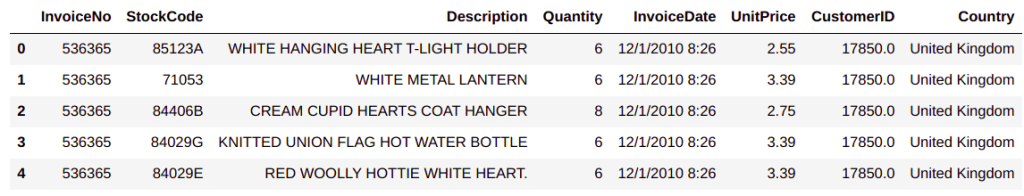
The above function reads the csv file and returns the data frame. Let us use this function to load the data and view the head of the data
# Please define your specific path where the data set is loaded
filename = "OnlineRetail.csv"
# Let us load the customer Details
custDetails = dataLoader(filename)
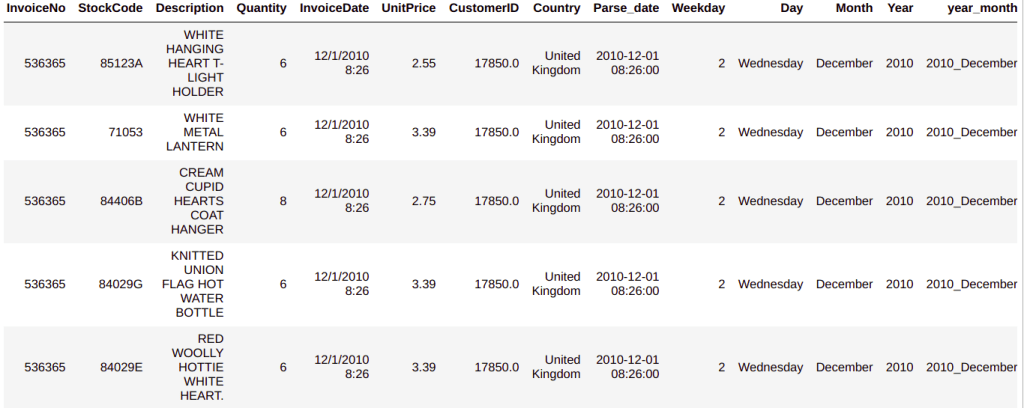
custDetails.head()
Further in the exercise we have to work a lot with the dates and therefore we need to extract relevant details from the date column like the day, weekday, month, year etc. We will do that with the date parser library. Let us now parse all the date related column and create new columns storing the new details we extract after parsing the dates.
#Parsing  the date
custDetails['Parse_date'] = custDetails["InvoiceDate"].apply(lambda x: parse(x))
# Parsing the weekdaty
custDetails['Weekday'] = custDetails['Parse_date'].apply(lambda x: x.weekday())
# Parsing the Day
custDetails['Day'] = custDetails['Parse_date'].apply(lambda x: x.strftime("%A"))
# Parsing the Month
custDetails['Month'] = custDetails['Parse_date'].apply(lambda x: x.strftime("%B"))
# Extracting the year
custDetails['Year'] = custDetails['Parse_date'].apply(lambda x: x.strftime("%Y"))
# Combining year and month together as one feature
custDetails['year_month'] = custDetails['Year'] + "_" +custDetails['Month']

custDetails.head()
As seen from line 22 we have used the lambda() function to first parse the ‘date’ column. The parsed date is stored in a new column called ‘Parse_date’. After parsing the dates first, we carry out different operations, again using the lambda() function on the parsed date. The different operations we carry out are
- Extract weekday and store it in a new column called ‘Weekday’ : line 24
- Extract the day of the week and store it in the column ‘Day’ : line 26
- Extract the month and store in the column ‘Month’ : line 28
- Extract year and store in the column ‘Year’ : line 30
Finally, in line 32 we combine the year and month to form a new column called ‘year_month’. This is done to enable easy filtering of data based on the combination of a year and month.
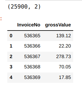
We will also create a column which gives you the gross value of each puchase. Gross value can be calculated by multiplying the quantity with unit price.
# Creating gross value column
custDetails['grossValue'] = custDetails["Quantity"] * custDetails["UnitPrice"]
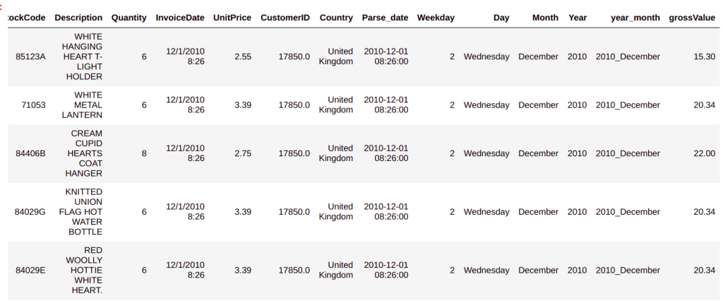
custDetails.head()
The reason we are calculating the gross value is to use it for segmentation of customers which will be dealt with in the next section. This takes us to the end of the initial preparation of the data set. Next we start creating customer segments.
Creating Customer Segments
In the last post, where we formulated the problem statement, we identified that customer segment could be one of the important components of the states. In addition to the customer segment,the other components are day of purchase and period of the month. So our next endeavour is to prepare data to create the different states we require. We will start with defining the customer segment.
There are different approaches to creating customer segments. In this post we will use the RFM analysis to create customer segments. Let us get going with creation of customer segments from our data set. We will continue on the same notebook we were using so far.
import lifetimes
In line 39,We import the lifetimes package to create the RFM data from our transactional dataset. Next we will use the package to convert the transaction data to the specific format.
# Converting data to RFM format
RfmAgeTrain = lifetimes.utils.summary_data_from_transaction_data(custDetails, 'CustomerID', 'Parse_date', 'grossValue')
RfmAgeTrain
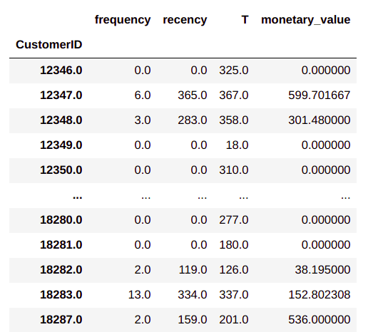
The process for getting the frequency, recency and monetary value is very simple using the life time package as shown in line 42 . From the output we can see the RFM data frame formed with each customer ID as individual row. For each of the customer, the frequency and recency in days is represented along with the average monetary value for the customer. We will be using these values for creating clusters of customer segments.
Before we work further, let us clean the data frame a bit by resetting the index values as shown in line 44
RfmAgeTrain = RfmAgeTrain.reset_index()
RfmAgeTrain

What we will now do is to use recency, frequency and monetary values seperately to create clusters. We will use the K-means clustering technique to find the number of clusters required. Many parts of the code used for clustering is taken from the following post on customer segmentation.
In lines 46-47 we import the Kmeans clustering method and matplotlib library.
from sklearn.cluster import KMeans
import matplotlib.pyplot as plt
For the purpose of getting the recency matrix let us take a subset of the data frame with only customer ID and recency value as shown in lines 48-49
user_recency = RfmAgeTrain[['CustomerID','recency']]
user_recency.head()

In any clustering problem,as you might know, one of the critical tasks is to determine the number of clusters which in the Kmeans algorithm is a parameter. We will use the well known elbow method to find the optimum number of clusters.
# Initialize a dictionary to store sum of squared error
sse = {}
recency = user_recency[['recency']]

# Loop through different cluster combinations
for k in range(1,10):
    # Fit the Kmeans model using the iterated cluster value
    kmeans = KMeans(n_clusters=k,max_iter=2000).fit(recency)
    # Store the cluster against the sum of squared error for each cluster formation
    sse[k] = kmeans.inertia_

# Plotting all the clusters
plt.figure()
plt.plot(list(sse.keys()),list(sse.values()))
plt.xlabel("Number of clusters")
plt.show()
In line 51, we initialise a dictionary to store the sum of square error for each k-means cluster and then subset the data frame ‘recency’ with only the recency values in line 52.
From line 55, we start a loop to itrate through different cluster values. For each cluster value, we fit the k-means model in line 57. We also store the sum of squared error in line 59 for each of the cluster in the dictionary we initialized.
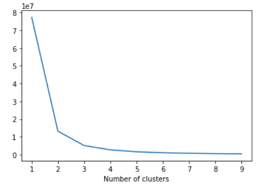
Lines 62-65, we visualise the number of clusters against the sum of squared error, which gives and indication of the right k value to choose.
From the plot we can see that 2,3 and 4 cluster values are where the elbow tapers and one of these values can be taken as the cluster value.Let us choose 4 clusters for our purpose and then refit the data.
# let us take four clusters
kmeans = KMeans(n_clusters=4)
# Fit the model on the recency data
kmeans.fit(user_recency[['recency']])
# Predict the clusters for each of the customer
user_recency['RecencyCluster'] = kmeans.predict(user_recency[['recency']])
user_recency
In line 67, we instantiate the KMeans class using 4 clusters. We then use the fit method on the recency values in line 69. Once the model is fit, we predict the cluster for each customer in line 71.
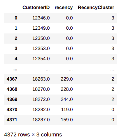
From the output we can see that the recency cluster is predicted against each customer ID. We will clean up this data frame a bit, by resetting the index.
user_recency.sort_values(by='recency',ascending=False).reset_index(drop=True)

From the output we can see that the data is ordered according to the clusters. Let us also look at how the clusters are mapped vis a vis the actual recency value. For doing this, we will group the data with respect to each cluster and then find the mean of the recency value, as in line 74.
user_recency.groupby('RecencyCluster')['recency'].mean().reset_index()

From the output we see the mean value of recency for each cluster. We can clearly see that there is a demarcation of the mean values with the value of the cluster. However, the mean values are not mapped in a logical (increasing or decreasing) order of the clusters. From the output we can see that cluster 3 is mapped to the smallest recency value ( 7.72). The next smallest value (115.85) is mapped to cluster 0 and so on. So there is not specific ordering to the custer and the mean value mapping. This might be a problem when we combine all the clusters for recency, frequency and monetary together to derive a combined score. So it is necessary to sort it in an ordered fashion. We will use a custom function to get the order right. Let us see the function.
# Function for ordering cluster numbers

def order_cluster(cluster_field_name,target_field_name,data,ascending):
    # Group the data on the clusters and summarise the target field(recency/frequency/monetary) based on the mean value
    data_new = data.groupby(cluster_field_name)[target_field_name].mean().reset_index()
    # Sort the data based on the values of the target field
    data_new = data_new.sort_values(by=target_field_name,ascending=ascending).reset_index(drop=True)
    # Create a new column called index for storing the sorted index values
    data_new['index'] = data_new.index
    # Merge the summarised data onto the original data set so that the index is mapped to the cluster
    data_final = pd.merge(data,data_new[[cluster_field_name,'index']],on=cluster_field_name)
    # From the final data drop the cluster name as the index is the new cluster
    data_final = data_final.drop([cluster_field_name],axis=1)
    # Rename the index column to cluster name
    data_final = data_final.rename(columns={'index':cluster_field_name})
    return data_final
In line 77, we define the function and its inputs. Let us look at the inputs to the function
cluster_field_name : This is the field name we give to the cluster in the data set like “RecencyCluster”.
target_field_name : This is the field pertaining to our target values like ‘recency’ , ‘frequency’ and ,’monetary_values’.
data : This is the data frame containing the cluster information and target values, for eg ( user_recency)
ascending : This is a flag indicating whether the data has to be sorted in ascending order or not
Line 79, we group the data based on the cluster and summarise the data under each group to get the mean of the target variable. The idea is to sort the data frame based on the mean values in ascending order which is done in line 81. Once the data is sorted in ascending order, we form a new feature with the data frame index as its values, in line 83. Now the index values will act as sorted cluster values and we will get a mapping between the existing cluster values and the new cluster values which are sorted. In line 85, we merge the summarised data frame with the original data frame so that the new cluster values are mapped to all the values in the data frame. Once the new sorted cluster labels are mapped to the original data frame, the old cluster labels are dropped in line 87 and the column renamed in line 89
Now that we have defined the function, let us implement it and sort the data frame in a logical order in line 91.
user_recency = order_cluster('RecencyCluster','recency',user_recency,False)
Next we will summarise the new sorted data frame and check if the clusters and mapped in a logical order.
user_recency.groupby('RecencyCluster')['recency'].mean().reset_index()

From the above output we can see that the cluster numbers are mapped in a logical order of decreasing recency.
We now need to repeat the process for frequency and monetary values. For convenience we will wrap all these processes in a new function.
def clusterSorter(target_field_name,ascending):
    # Make the subset data frame using the required feature
    user_variable = RfmAgeTrain[['CustomerID',target_field_name]]
    # let us take four clusters indicating 4 quadrants
    kmeans = KMeans(n_clusters=4)
    kmeans.fit(user_variable[[target_field_name]])
    # Create the cluster field name from the target field name
    cluster_field_name = target_field_name + 'Cluster'
    # Create the clusters
    user_variable[cluster_field_name] = kmeans.predict(user_variable[[target_field_name]])
    # Sort and reset index
    user_variable.sort_values(by=target_field_name,ascending=ascending).reset_index(drop=True)
    # Sort the data frame according to cluster values
    user_variable = order_cluster(cluster_field_name,target_field_name,user_variable,ascending)
    return user_variable
Let us now implement this function to get the clusters for frequency and monetary values.
# Implementing for user frequency
user_freqency = clusterSorter('frequency',True)
user_freqency.groupby('frequencyCluster')['frequency'].mean().reset_index()

# Implementing for monetary values
user_monetary = clusterSorter('monetary_value',True)
user_monetary.groupby('monetary_valueCluster')['monetary_value'].mean().reset_index()

Let us now sit back and look at the three results which we got and try to analyse the results. For recency, we implemented the process using ‘ascending’ value as ‘False’ and the other two with ascending value as ‘True’. Why do you think we did it this way ?
To answer let us look these three variables from the perspective of the desirable behaviour from a customer. We would want customers who are very recent, are very frequent and spent lot of money. So from a recency perspective lesser days is a good behaviour as this indicate very recent customers. The reverse is true for frequency and monetary where the more of those values is the desirable behaviour. This is why we used 'ascending = false' in the recency variable as the clusters would be sorted with the less frequent ( more days) for cluster ‘0’ and the mean days comes down when we go to cluster 3. So in effect we are making cluster 3 as the group of most desirable customers. The reverse applies to frequency and monetary value where we gave 'ascending = True' to make custer 3 as the group of most desirable customers.
Now that we have obtained the clusters for each of the variables seperately, its time to combine them into one data frame and then get a consolidated score which will become the segments we want.
Let us first combine each of the individual dataframes we created with the original data frame
# Merging the individual data frames with the main data frame
RfmAgeTrain = pd.merge(RfmAgeTrain,user_monetary[["CustomerID",'monetary_valueCluster']],on='CustomerID')
RfmAgeTrain = pd.merge(RfmAgeTrain,user_freqency[["CustomerID",'frequencyCluster']],on='CustomerID')
RfmAgeTrain = pd.merge(RfmAgeTrain,user_recency[["CustomerID",'RecencyCluster']],on='CustomerID')
RfmAgeTrain.head()
In lines 115-117, we combine the individual dataframes to our main dataframe. We combine them on the ‘CustomerID’ field. After combining we have a consolidated data frame with each individual cluster label mapped to each customer id as shown below

Let us now add the individual cluster labels to get a combined cluster score.
# Calculate the overall score
RfmAgeTrain['OverallScore'] = RfmAgeTrain['RecencyCluster'] + RfmAgeTrain['frequencyCluster'] + RfmAgeTrain['monetary_valueCluster']
RfmAgeTrain

Let us group the data based on the ‘OverallScore’ and find the mean values of each of our variables , recency, frequency and monetary.
RfmAgeTrain.groupby('OverallScore')['frequency','recency','monetary_value'].mean().reset_index()
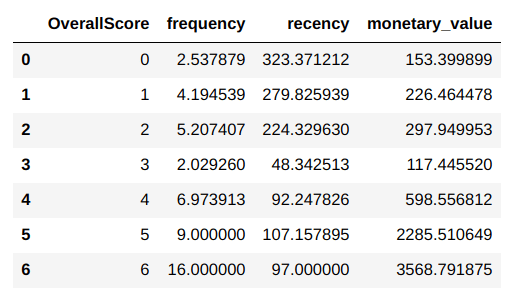
From the output we can see how the distributions of the new clusters are. From the values we can see that there is some level of logical demarcation according to the cluster labels. The higher cluster labels ( 4,5 & 6) have high monetary values, high frequency levels and also mid level recency levels. The first two clusters ( 0 & 1) have lower monetary values, high recency and low levels of frequency. Another stand out cluster is cluster 3, which has the lowest monetary value, lowest frequency and the lowest recency. We can very well go with these six clusters or we can combine clusters who demonstrate similar trends/behaviours. However this assessment needs to be taken based on the number of customers we have under each of these new clusters. Let us get those numbers first.
RfmAgeTrain.groupby('OverallScore')['frequency'].count().reset_index()
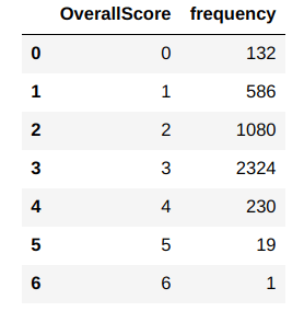
From the counts, we can see that the higher scores ( 4,5,6) have very few customers relative to the other clusters. So it would make sense to combine them to one single segment. As these clusters have higher values we will make them customer segment ‘Q4’. Cluster 3 has some of the lowest relative scores and so we will make it segment ‘Q1’. We can also combine clusters 0 & 1 to a single segment as the number of customers for those two clusters are also lower and make it segment ‘Q2’. Finally cluster 2 would be segment ‘Q3’ . Lets implement these steps next.
RfmAgeTrain['Segment'] = 'Q1'
RfmAgeTrain.loc[(RfmAgeTrain.OverallScore == 0) ,'Segment']='Q2'
RfmAgeTrain.loc[(RfmAgeTrain.OverallScore == 1),'Segment']='Q2'
RfmAgeTrain.loc[(RfmAgeTrain.OverallScore == 2),'Segment']='Q3'
RfmAgeTrain.loc[(RfmAgeTrain.OverallScore == 4),'Segment']='Q4'
RfmAgeTrain.loc[(RfmAgeTrain.OverallScore == 5),'Segment']='Q4'
RfmAgeTrain.loc[(RfmAgeTrain.OverallScore == 6),'Segment']='Q4'

RfmAgeTrain

After allocating the clusters to the respective segments, the subsequent data frame will look as above. Let us now take the mean values of each of these segments to understand how the segment values are distributed.
RfmAgeTrain.groupby('Segment')['frequency','recency','monetary_value'].mean().reset_index()

From the output we can see that for each customer segment the monetary value and frequency values are in ascending order. The value of recency is not ordered in any fashion. However that dosent matter as all what we are interested in getting is the segmentation of the customer data into four segments. Finally let us merge the segment information to the orginal customer transaction data.
# Merging the customer details with the segment
custDetails = pd.merge(custDetails, RfmAgeTrain, on=['CustomerID'], how='left')
custDetails.head()

The above output is just part of the final dataframe. From the output we can see that the segment data is updated to the original data frame.
With that we complete the first step of our process. Let us summarise what we have achieved so far.
- Preprocessed data to extract information required to generate states
- Transformed data to the RFM format.
- Clustered data with respect to recency, frequency and monetary values and then generated the composite score.
- Derived 4 segments based on the cluster data.
Having completed the segmentation of customers, we are all set to embark on the most important processes.
What Next ?
The next step is to take the segmentation information and then construct our states and action strategies from them. This will be dealt with in the next post. Let us take a peek into the processes we will implement in the next post.
- Create states and actions from the customer segments we just created
- Initialise the value distribution and rewards distribution
- Build the self learning recommendaton system using the epsilon greedy method
- Simulate customer action to get the feed backs
- Update the value distribution based on customer feedback and improve recommendations
There is lot of ground which will be covered in the next post.Please subscribe to this blog post to get notifications when the next post is published.
You can also subscribe to our Youtube channel for all the videos related to this series.
The complete code base for the series is in the Bayesian Quest Git hub repository
Do you want to Climb the Machine Learning Knowledge Pyramid ?
Knowledge acquisition is such a liberating experience. The more you invest in your knowledge enhacement, the more empowered you become. The best way to acquire knowledge is by practical application or learn by doing. If you are inspired by the prospect of being empowerd by practical knowledge in Machine learning, subscribe to our Youtube channel
I would also recommend two books I have co-authored. The first one is specialised in deep learning with practical hands on exercises and interactive video and audio aids for learning
This book is accessible using the following links
The Deep Learning Workshop on Amazon
The Deep Learning Workshop on Packt
The second book equips you with practical machine learning skill sets. The pedagogy is through practical interactive exercises and activities.

This book can be accessed using the following links
The Data Science Workshop on Amazon
The Data Science Workshop on Packt
Enjoy your learning experience and be empowered !!!!