Building Self Learning Recommendation system – III : Recommendation System as a K-armed Bandit

This is the third post of our series on building a self learning recommendation system using reinforcement learning. This series consists of 8 posts where in we progressively build a self learning recommendation system.

Recommendation system and reinforcement learning primer
Introduction to multi armed bandit problem
Self learning recommendation system as a K-armed bandit ( This post )
Build the prototype of the self learning recommendation system: Part I
Build the prototype of the self learning recommendation system: Part II
Productionising the self learning recommendation system: Part I – Customer Segmentation
Productionising the self learning recommendation system: Part II – Implementing self learning recommendation
Evaluating different deployment options for the self learning recommendation systems.

Introduction

In our previous post we implemented couple of experiments with K-armed bandit. When we discussed the idea of the K-armed bandits from the context of recommendation systems, we briefly touched upon the idea that the buying behavior of a customer depends on the customers context. In this post we will take the idea of the context forward and how the context will be used to build the recommendation system using the K-armed bandit solution.

Defining the context for customer buying

When we discussed about reinforcement learning in our first post, we learned about the elements of a reinforcement learning setting like state, actions, rewards etc. Let us now identify these elements in the context of the recommendation system we are building.

State

When we discussed about reinforcement learning in the first post, we learned that when an agent interacts with the environment at each time step, the agent manifests a certain state. In the example of the robot picking trash the different states were that of high charge or low charge. However in the context of the recommendation system, what would be our states ? Let us try to derive the states from the context of a customer who makes an online purchase. What would be those influencing factors which defines the product the customer buys ? Some of these are

The segment the customer belongs
The season or time of year the purchase is made
The day in which purchase is made

There could be many other influencing factors other than this. For simplicity let us restrict to these factors for now. A state could be made from the combinations of all these factors. Let us arrive at these factors through some exploratory analysis of the data

The data set we would be using is the online retail data set available in the UCI Machine learning library. We will download the data and the place it in local folder and the read the file from the local folder.

import numpy as np
import pandas as pd
from dateutil.parser import parse

Lines 1-3 imports all the necessary packages for our purpose. Let us now load the data as a pandas data frame

# Please use the path to the actual data
filename = "data/Online Retail.xlsx"
# Let us load the customer Details
custDetails = pd.read_excel(filename, engine='openpyxl')
custDetails.head()

In line 5, we load the data from disk and then read the excel shee using the ‘openpyxl’ engine. Please note to pip install the ‘openpyxl’ package if not available.

Let us now parse the date column using date parser and extract information from the date column.

#Parsing  the date
custDetails['Parse_date'] = custDetails["InvoiceDate"].apply(lambda x: parse(str(x)))
# Parsing the weekdaty
custDetails['Weekday'] = custDetails['Parse_date'].apply(lambda x: x.weekday())
# Parsing the Day
custDetails['Day'] = custDetails['Parse_date'].apply(lambda x: x.strftime("%A"))
# Parsing the Month
custDetails['Month'] = custDetails['Parse_date'].apply(lambda x: x.strftime("%B"))
# Getting the year
custDetails['Year'] = custDetails['Parse_date'].apply(lambda x: x.strftime("%Y"))
# Getting year and month together as one feature
custDetails['year_month'] = custDetails['Year'] + "_" +custDetails['Month']
# Feature engineering of the customer details data frame
# Get the date  as a seperate column
custDetails['Date'] = custDetails['Parse_date'].apply(lambda x: x.strftime("%d"))
# Converting date to float for easy comparison
custDetails['Date']  = custDetails['Date'] .astype('float64')
# Get the period of month column
custDetails['monthPeriod'] = custDetails['Date'].apply(lambda x: int(x > 15))

custDetails.head()

As seen from line 11 we have used the lambda() function to first parse the ‘date’ column. The parsed date is stored in a new column called ‘Parse_date’. After parsing the dates first, we carry out different operations, again using the lambda() function on the parsed date. The different operations we carry out are

Extract weekday and store it in a new column called ‘Weekday’ : line 13
Extract the day of the week and store it in the column ‘Day’ : line 15
Extract the month and store in the column ‘Month’ : line 17
Extract year and store in the column ‘Year’ : line 19

In line 21 we combine the year and month to form a new column called ‘year_month’. This is done to enable easy filtering of data, based on the combination of a year and month.

We make some more changes from line 24-28. In line 24, we extract the date of the month and then convert it into a float type in line 26. The purpose of taking the date is to find out which of these transactions have happened before 15th of the month and which after 15th. We extract those details in line 28, where we create a binary points ( 0 & 1) as to whether a date falls in the last 15 days or the first 15 days of the month.

We will also create a column which gives you the gross value of each puchase. Gross value can be calculated by multiplying the quantity with unit price. After that we will consolidate the data for each unique invoice number and then explore some of the elements of states which we want to explore

# Creating gross value column
custDetails['grossValue'] = custDetails["Quantity"] * custDetails["UnitPrice"]
# Consolidating accross the invoice number for gross value
retailConsol = custDetails.groupby('InvoiceNo')['grossValue'].sum().reset_index()
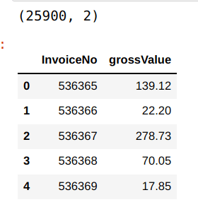
print(retailConsol.shape)
retailConsol.head()

Now that we have got the data consolidated based on each invoice number, let us merge the date related features from the original data frame with this consolidated data. We merge the consolidated data with the custDetails data frame and then drop all the duplicate data so that we get a record per invoice number, along with its date features.

# Merge the other information like date, week, month etc
retail = pd.merge(retailConsol,custDetails[["InvoiceNo",'Parse_date','Weekday','Day','Month','Year','year_month','monthPeriod']],how='left',on='InvoiceNo')
# dropping ALL duplicate values
retail.drop_duplicates(subset ="InvoiceNo",keep = 'first', inplace = True)
print(retail.shape)
retail.head()

Let us first look at the month wise consolidation of data and then plot the data. We will use a functions to map the months to its index position. This is required to plot the data according to months. The function ‘monthMapping‘, maps an integer value to the month and then sort the data frame.

# Create a map for each month
def monthMapping(mnthTrend):
    # Get the map
    mnthMap = {"January": 1, "February": 2,"March": 3, "April": 4,"May": 5, "June": 6,"July": 7, "August": 8,"September": 9, "October": 10,"November": 11, "December": 12}
    # Create a new feature for month
    mnthTrend['mnth'] = mnthTrend.Month
    # Replace with the numerical value
    mnthTrend['mnth'] = mnthTrend['mnth'].map(mnthMap)
    # Sort the data frame according to the month value
    return mnthTrend.sort_values(by = 'mnth').reset_index()

We will use the above function to consolidate the data according to the months and then plot month wise grossvalue data

mnthTrend = retail.groupby(['Month'])['grossValue'].agg('mean').reset_index().sort_values(by = 'grossValue',ascending = False)
# sort the months in the right order
mnthTrend = monthMapping(mnthTrend)
sns.set(rc = {'figure.figsize':(20,8)})
sns.lineplot(data=mnthTrend, x='Month', y='grossValue')
plt.legend(bbox_to_anchor=(1.02, 1), loc='upper left', borderaxespad=0)
plt.show()

We can see that there is sufficient amount of variability of data month on month. So therefore we will take months as one of the context items on which the states can be constructed.

Let us now look at buying pattern within each month and check how the buying pattern is within the first 15 days and the latter half

# Aggregating data for the first 15 days and latter 15 days
fortnighTrend = retail.groupby(['monthPeriod'])['grossValue'].agg('mean').reset_index().sort_values(by = 'grossValue',ascending = False)

sns.set(rc = {'figure.figsize':(20,8)})
sns.lineplot(data=fortnighTrend, x='monthPeriod', y='grossValue')
plt.legend(bbox_to_anchor=(1.02, 1), loc='upper left', borderaxespad=0)
plt.show()

We can see that there is as small difference between buying patterns in the first 15 days of the month and the latter half of the month. Eventhough the difference is not significant, we will still take this difference as another context.

Next let us aggregate data as per the days of the week and and check the trend

# Aggregating data accross weekdays
dayTrend = retail.groupby(['Weekday'])['grossValue'].agg('mean').reset_index().sort_values(by = 'grossValue',ascending = False)

sns.set(rc = {'figure.figsize':(20,8)})
sns.lineplot(data=dayTrend, x='Weekday', y='grossValue')
plt.legend(bbox_to_anchor=(1.02, 1), loc='upper left', borderaxespad=0)
plt.show()

We can also see that there is quite a bit of variability of buying patterns accross the days of the week. We will therefore take the week days also as another context

So far we have observed 4 different features, which will become our context for recommending products. The context which we have defined would act as the states from the reinforcement learning setting perspective. Let us now look at the big picture of how we will formulate the recommendation task as reinforcement learning setting.

The Big Picture

We will now have a look at the big picture of this implementation. The above figure is the representation of what we will implement in code in the next few posts.

The process starts with the customer context, consisting of segment, month, period in the month and day of the week. The combination of all the contexts will form the state. From an implementation perspective we will run simulations to generate the context since we do not have a real system where customers logs in and thereby we automatically capture context.

Based on the context, the system will recommend different products to the customer. From a reinforcement learning context these are the actions which are taken from each state. The initial recommendation of products ( actions taken) will be based on the value function learned from the historical data.

The customer will give rewards/feedback based on the actions taken( products recommended ). The feedback would be the manifestation of the choices the customer make. The choice the customer makes like the products the customer buys, browses and ignores from the recommended list. Depending on the choice made by the customer, a certain reward will be generated. Again from an implementation perspective, since we do not have real customers giving feedback, we will be simulating the customer feedback mechanism.

Finally the update of the value functions based on the reward generated will be done based on the simple averaging method. Based on the value update, the bandit will learn and adapt to the affinities of the customers in the long run.

What next ?

In this post we explored the data and then got a big picture of what we will implement going forward. In the next post we will start implementing these processes and building a prototype using Jupyter notebook. Later on we will build an application using Python scripts and then explore options to deploy the application. Watch out this space for more.

The next post will be published next week. Please subscribe to this blog post to get notifications when the next post is published.

You can also subscribe to our Youtube channel for all the videos related to this series.

The complete code base for the series is in the Bayesian Quest Git hub repository

Do you want to Climb the Machine Learning Knowledge Pyramid ?

Knowledge acquisition is such a liberating experience. The more you invest in your knowledge enhacement, the more empowered you become. The best way to acquire knowledge is by practical application or learn by doing. If you are inspired by the prospect of being empowerd by practical knowledge in Machine learning, subscribe to our Youtube channel

I would also recommend two books I have co-authored. The first one is specialised in d eep learning with practical hands on exercises and interactive video and audio aids for learning

This book is accessible using the following links

The Deep Learning Workshop on Amazon

The Deep Learning Workshop on Packt

The second book equips you with practical machine learning skill sets. The pedagogy is through practical interactive exercises and activities.

This book can be accessed using the following links

The Data Science Workshop on Amazon

The Data Science Workshop on Packt

Enjoy your learning experience and be empowered !!!!

Building Self learning Recommendation System using Reinforcement Learning : Part I

In our previous series on building data science products we learned how to build a machine translation application and how to deploy the application. In this post we start a new series where in we will build a self learning recommendation system. We will be building this system using reinforcement learning methods. We will be leveraging the principles of the bandit problem to build our self learning recommendation engine. This series will be split across 8 posts.

Let us start our series with a primer on Recommendations systems and Reinforcement learning.

Primer on Recommendation Systems

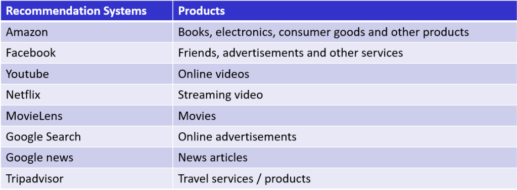
Recommendation systems (RS) are omnipresent phenomenon which we encounter in our day to day life. Powering the modern day e-commerce systems are gigantic ‘recommendation engines’, looking at each individual transactions, mapping customer profiles and using them to recommend personalized products and services.

Before we embark on building our self learning recommendation system, it will be a good idea to take a quick tour on different types of recommendation systems powering large e-commerce systems of the modern era.

For convenience let us classify recommendation systems into three categories,

Figure 1 : Different types of Recommendation Systems

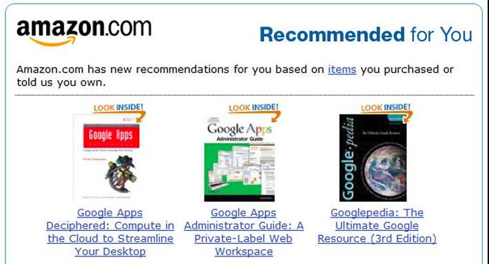
Traditional recommendation systems leverages data involving user-item interactions ( buying behavior of users ,ratings given by users, etc. ) and attribute information of items ( textual descriptions of items ). Some of the popular type of recommendation systems under the traditional umbrella are

Collaborative Filtering Recommendation Systems : The fundamental principle behind collaborative filtering systems is that, two or more individuals who share similar interests tend to have similar propensities for buying. The similarity between individuals are unearthed using the ratings they give, their browsing patterns or their buying patterns. There are different types of collaborative filtering systems like user-based collaborative filtering, item-based collaborative filtering, model based methods ( decision trees, Bayesian models, latent factor models ),etc.

Figure 2 : Collaborative filtering Recommendation Systems

Content Based Recommendation Systems : In content based recommendation systems, attribute descriptions of the items are the basis of recommendations. For example if you are a person who watched the Jason Borne series movies and haven’t given any ratings, content based recommendation systems would infer your tastes from the attributes of the movies you watched like action thriller ,CIA , covert operations etc. Based on these attributes the system would recommend movies like Mission Impossible series, as they follow a similar genre.

Figure 3 : Content Based Recommendation Systems

Knowledge Based Recommendation Systems : These type of systems make recommendations based on similarity between a users requirements and an item descriptions. Knowledge based recommendation systems are usually useful in context where the purchases infrequent like buying an automobile, real estate, luxury goods etc.

Figure 4 : Knowledge Based Recommendation System

Hybrid Recommendation Systems : Hybrid systems or Ensemble systems as they might be called combine best features of the above mentioned approaches to generate recommendations. For example Netflix uses a combination of collaborative filtering ( based on user ratings) and content based( attribute descriptions of movies) to make recommendations.

Traditional class of recommendation systems like collaborative filtering are predominantly linear in its approach. However personalization of customer preferences are not necessarily linear and therefore there was need for modelling recommendation systems for behavior data which are mostly non linear and this led to the rise of deep learning based systems. There are many proponents of deep learning methods some of the notable ones are Youtube, ebay, Twitter and Spotify. Let us now see some of the most popular types of deep learning based recommendation systems.

Multi Layer Perceptron based Recommendation Systems : Multi layer perceptron or MLP based recommendation systems are feed-forward neural network systems with multiple layers between the input layer and output layer. The basic setting for this approach is to vectorize user information and item information as the basic inputs. This input layer is fed into the feed forward network and then the output is whether there is an interaction for the item or not. By modelling these interactions as a MLP we will be able to rank specific products in terms of the propensity of the user to that item.

Figure 5: MLP Based Recommendation System

CNN based Recommendation Systems : Convolutional Neural networks ( CNN ) are great feature extractors, i.e. they extract global level and local level features. These features are used for providing context which will aid in better recommendations.

RNN based Recommendation System: RNNs are good choices when there are sequences of data. In the context of a recommendation systems use cases like recommending what the user will click next can be treated as a sequence to sequence problem. In such problems the interactions between the user and an item at each session will be the basic data and the output will be what the customer clicked next. So if we have data pertaining to session information and the interaction of the user to items during the sessions, we will be able to model a RNN to be used as a Recommender system.
Neural attention based Recommendation Systems : Attention based recommendation systems leverage the attention mechanism which has great utility in use cases like machine translation, image captioning, to name a few. Attention based recommendation systems are more apt for recommending multimedia items like photos and videos. In multimedia recommendation, the user preferences can be implicit ( likes, views ). These implicit feed back need not always mean that a user liked that item. For example I might give a like to a video or photo shared by a friend even if I really don’t like those items. In such cases, attention based models attempt to weight the user-item interactions to give more emphasis to parts of the video or image which could be more aligned to the users preferences.

Figure 6 : Deep Learning Based Recommendation System ( Image source : dzone.com/articles/building-a-recommendation-system-using-deep-learni)

The above are some of the prevalent deep learning based recommendation systems. In addition to these there are other deep learning algorithms like Restricted Boltzmann machines based recommendation systems , Autoencoder based recommendation systems and Neural autoregressive recommendation systems . We will explore creation of recommendation systems with these types of models in a future post. Deep learning methods for recommendation systems have tremendous abilities to model non linear relationships between user interactions with items. However on the flip side, there is a severe problem of interpretability of models and the hunger for more data in deep learning methods. Off late deep reinforcement learning methods are widely used as recommendation systems. Deep reinforcement learning systems have abilities to model with large number of states and action spaces and this has made reinforcement learning methods to be used as recommendation systems. Let us explore some of the prominent types of reinforcement learning based recommendation systems.

Since this series is about the application of reinforcement learning to the application of recommendation systems, let us first understand what reinforcement learning is and then get into application of reinforcement learning as recommendation systems.

Primer on Reinforcement Learning

Unlike the supervised learning setting where there is a guide telling you what the right action is, reinforcement learning relies on the environment to discover what the right action is. The learning in reinforcement learning is through interaction with an environment. In the reinforcement learning setting there is an agent ( recommendation system in our context) which receives rewards ( feed back from users like buying, clicking) from the environment ( users ) . The rewards acts as an indicator as to whether the course of action taken by the agent is right or wrong. The agent ultimately learns to take the right action through feed backs received from the environment over a period of time.

Figure 7 : Reinforcement Learning Setting

Elements of Reinforcement Learning

Let us try to understand different elements of reinforcement learning with an example of a robot picking trash.

We will first explore an element of reinforcement learning called the ‘State’. A state can be defined as the representation of the environment in which a task has to be performed. In the context of our robot, we can say that it has two states.

State 1 : High charge

State 2 : Low charge.

Depending on the state the robot is in, it has three decision points to make.

The robot can go on searching for trash.
The robot can wait at its current location so that some one will pick up trash and give it to the robot
The robot can got to its charging station to recharge so that it doesn’t go off power.

These decision points which are taken at each state is called an ‘Action‘ in reinforcement learning parlance.

Let us represent the states and its corresponding actions for our robot

From the above figure we can observe the states of the robot and the actions the robot can take. When the robot has high charge, there would only be two actions the robot is likely to take as there would be no point in recharging as the current charge is high.

Depending on the current state and the action taken from that state, the robot will transition to the next state. Let us look at some possible states the robot can end up based on the initial state and the action it takes.

State : High Charge ,Action : Search

When the current state is high charge and the action taken is search, there are two possible states the robot can attain, stay in its high charge( because the search was quickly over) or deplete its charge and end up with low charge.

State : High Charge ,Action : Wait

If the robot decides to wait when it is high on charge, the robot continues in its state of high charge.

State : Low Charge ,Action : Search

When the charge is low and the robot decides to search there can be two resultant states. One plausible scenario is for the charge to be completely drained making the robot unable to take further action. In such circumstance someone will have to physically take the robot to the charging point and the robot ends up with high charge.

The second scenario is when the robot do not make extensive search and as a result doesn’t drain much. In this scenario the robot continues in its state of low charge.

State : Low Charge ,Action : Wait

When the action is to wait with low charge the robot continues to remain in a state of low charge.

State : Low Charge ,Action : Recharge

Recharging the robot will enable the robot to return to a state of high charge.

Based on our discussions let us now represent the states, different action choices and the subsequent states the robot will end up

So far we have seen different starting states and subsequent states the robot ends up based on the action choices the robot makes. However, what about the consequences for the different action choices the robot makes ? We can see that there are some desirable consequences and some undesirable consequences. For example remaining in high charge state by searching for trash is a desirable consequence. However draining off its charge is an undesirable consequence. To optimize the behavior of the robot we need to encourage desirable consequences and strictly discourage undesirable tendencies. How do we inculcate desirable tendencies and discourage undesirable ones ? This is where the concept of rewards comes in.

The sole purpose of the robot is to collect as much trash as possible. This purpose can be effectively done only when the robot searches for trash. However in the process of searching for trash the robot is also supposed to take care of itself i.e. it should ensure that it has enough charge to go about the search so that it doesn’t drain of charge and make itself ineffective. So the desired behavior for the robot is to search and collect trash and the undesired behavior is to get into a drained state. In order to inculcate the desired behaviors we can introduce rewards when the robot collects trash and also penalizes the robot when it drains itself of its charge. The other actions of waiting and recharging will not have any reward or penalties involved. This system of rewards will imbibe right behaviors in the robot.

The example we have seen of the robot is a manifestation of reinforcement learning. Let us now try to derive the elements of reinforcement learning from the context of the robot.

As seen from the robot example, reinforcement learning is the process of learning what to do at different scenarios based on feed back received. Within this context the part of the robot which learns and decides what to do is called the agent .

The context within which an agent interacts is called the environment. In the context of the robot, it is the space where the robot interacts in the process of carrying out its task of picking trash.

When the agent interacts with its environment, at each time step, the agent manifests a certain state. In our example we saw that the robot had two states of high charge and low charge.

From each state the agent carries out certain actions. The actions an agent carries out from a state will determine the subsequent state. In our context we saw how the actions like searching, waiting or recharging from a starting state defined the state the robot ended up.

The other important element is the reward function. The reward function quantifies the consequences of following certain actions from a state. The kind of reward an agent receives for a state-action pair defines the desirability of doing that action given its state. The objective of an agent is to maximize the rewards it gets in the long run.

The reward function is the quantification of the consequences which is got immediately after following a certain action. It doesn’t look far out in the future whether the course of action is good in the long term. That is what a value function does. A value function looks at maximizing the rewards which gets accumulated over a long term horizon. Imagine that the robot was in a state of low charge and then it spots some trash at a certain distance. So the robot decides to search and pick that trash as it would give an immediate reward. However in the process of searching and picking up the trash its charge drains off and the robot become ineffective, getting a large penalty in the process. In this case, even though the short term reward was good, the long term effect was harmful. If the robot had instead moved to its charging station to get charged and then gone in search of the trash, the overall value would have been more rewarding.

The next element of the reinforcement learning context is the policy. A policy defines how the agent has to behave at different circumstances at a given time. It guides the agent on what needs to be done depending on the circumstances. Let us revisit the situation we saw earlier on the decision point of the robot to recharge or to search for trash it spotted. Let us say there was a policy which said that the robot will have to recharge when the charge drops below a certain threshold. In such cases, the robot could have avoided the situation where the charge was drained. The policy is like the heart of the reinforcement learning context. The policy drives the behavior of agents at different situations.

An optional element of a reinforcement context is the model of the environment. A model is a broad representation of how an environment will behave. Given a state and the action taken from the state a model can be used to predict the next states and also the rewards which will be generated from those actions. A model is used for planning the course of action the agent has to take based on the situation the agent is in.

To sum up, we have seen that Reinforcement learning is a framework which aims at automating the task of learning and decision making. The automation of the learning and decision making process is achieved through the interaction between an agent and its environment through its various states, actions and rewards. The end objective of an agent is to maximize the value function and to learn a policy which maximizes the value function. We will be diving more deeper into some specific types of reinforcement learning problems in the future posts. Let us now look at some of the approaches to solve a reinforcement learning problem.

Different approaches using reinforcement learning

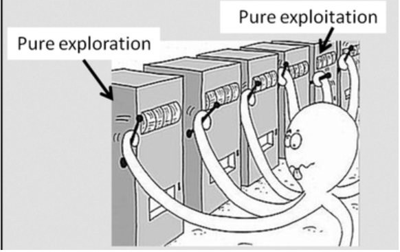
Multi-armed bandits : The name multi-armed bandits is derived from the context of a gambler who tries to maximize his/her returns by pulling multiple arms of a slot machine. The gambler through the process of exploration has to find which of the n arms provide the best rewards and once a set of best arms are identified, try to exploit those arms to maximize the rewards he/she gets from the process. In the context of reinforcement learning the problem can be formulated from the perspective of an agent who tries to get sufficient information of the environment ( different slots ) based on extensive exploration and then using the information gained to maximize the returns. Different use cases where multi armed bandits can be used involves clinical trials, recommendation systems, A/B testing, etc.

Figure 8 : Multi Armed Bandit – Exploration v/s Exploitation

Markov Decision Process and Dynamic Programming: Markov decision process falls under a class of algorithms called the model based algorithms. The main constituents of a Markov process involves the agent which interacts with the environment by taking actions from different states in which the agent finds itself. In a model based process there is a well defined probability distribution when going from one state to the other. This probability distribution is called the transition probability. The below figure depicts the transition probability of the robot we saw earlier. For example, if the robot is at state of low charge and it takes the action search, it would remain in the same state with probability and attains high charge with transition probability of 1-. Similarly, from a high state, when taking the action wait, the robot will remain in high charge with probability of 1.

Figure 9 : Markov Decision Process for a Robot ( Image source : Reinforcement Learning, Sutton & Barto )

Markov decision process entails that when moving from one state to the other, the history of all the states in which an agent was, doesn’t matter. All that matters is the current state. Markov decision processes are generally best implemented by a collection of algorithms called dynamic programming. Dynamic programming helps in computing the most optimal policies as a Markov decision process given a perfect model of the environment. What we mean by a perfect model of the environment is where we know all the states, actions and the transition probabilities when moving from one state to the other.

There are different use cases involving MDP process, some of the notable ones include determination of number of patients in a hospital, reducing wait time at intersections etc.

Monte Carlo Methods : Monte Carlo methods unlike dynamic programming and Markov decision processes, do not make assumptions on knowledge on the environment. Monte Carlo methods learns through experience. These methods rely on sampling sequences of states, actions and rewards to attain the most optimal solution.
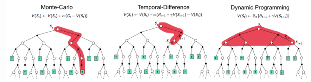
Temporal difference Methods : Temporal difference methods can be said as a combination of dynamic programming methods and Monte Carlo methods. Temporal difference methods can learn from experience like Monte Carlo methods and they also can also estimate the value function based on earlier learning without waiting for the end of an episode. Due to its simplicity temporal difference methods are great for learning experiences derived from interaction with environment in an online mode. Temporal difference methods are great to make long term predictions like predicting customer purchases, weather patterns, election outcomes etc.

Figure 10 : Comparison of backup diagram for MC,TD & DP ( Image source : David Silver’s RL Course, lecture 4 )

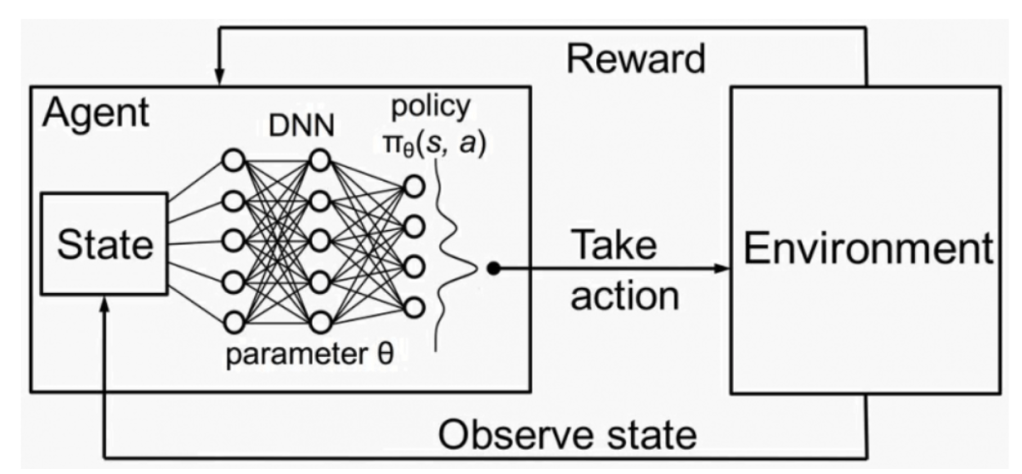
Deep Reinforcement Learning methods : Deep reinforcement learning methods combine traditional reinforcement learning and deep learning techniques. One pre-requisite of traditional reinforcement learning is the understanding of states and making decisions on what actions to take from each state. However reinforcement learning gets constrained when the number of states become very huge as in the case of many of the online data sets. This is where deep reinforcement learning techniques comes in handy. Deep reinforcement learning algorithms are able to take large input sets, which has large state spaces and make decisions on what actions to take to optimize the end objective. Deep reinforcement learning methods have wide applications in robotic, natural language processing, computer vision, finance, healthcare to name a few.

Having got an overview of the types of reinforcement learning systems, let us look at how reinforcement learning approaches can be used for building recommendation systems.

Reinforcement learning for recommendation systems

User interactions with items are sequential and it has a rich context to it. For this reason the problem of predicting the best item to a user can also be viewed as a sequential decision problem. In the primer on reinforcement systems, we learned that in a reinforcement learning setting, an agent aims to maximize a numerical reward through interactions with an environment. Bringing this to the recommendation system context, it is like the recommendation system (agent) trying to recommend an item ( an action ) to the user to maximize the user satisfaction ( reward ).

Let us now look at some of the approaches in which reinforcement learning is used as recommendation systems.

Multi armed bandit based recommendation systems : Recommendation systems can learn policies or decisions on what to recommend to whom by broadly two approaches. The first one is the traditional offline learning mode which we explored at the start of this article. The next approach is the online learning mode where the recommendation system will suggest an item to the user based on the users context like time of day, place, history, previous interactions etc. One of the basic type of systems which implement the online system is the multi armed bandit approach. This approach will basically treat the recommendation task like pulling the levers of an armed bandit.

Figure 12 : Multi-Armed Bandit as Recommendation System

Normal reinforcement learning based recommendation systems : Many of the reinforcement learning approaches which we explored earlier like MDP, Monte Carlo and Temporal Difference are widely used as recommendation systems. One such example is in the use of MDP based recommendation systems for recommending songs to users. In this problem setting the states represents the list of songs to be recommended, the action is the act of listening to songs, the transition probability is the probability of selecting a particular song having listened to a song and the reward is the implicit feed back received when the user actually listens to the recommended song.
Deep Reinforcement Learning based recommendation systems : Deep reinforcement learning systems have the ability to learn multiple states and action spaces. In a typical personalized online recommendation systems the number of states and actions are quite large and deep reinforcement learning systems are good fit for such use cases. Take the case of an approach to recommend movies based on a framework called Deep Deterministic Policy Gradient Framework. In this use case, user preferences are used to learn a policy which will thereby be used to select the movies to be recommended for the user. The learning of the policy is done using the deep deterministic policy gradient framework, which enables learning policies dynamically. The dynamic policy vector is then applied on the candidate set of movies to get a personalized set of movies to the user.

There are different use cases and multiple approaches to use reinforcement learning systems as recommendation systems. We will deal with more sophisticated reinforcement learning based recommendation systems in future posts.

What Next ?

So far in this post we have taken a quick overview of the main concepts. Obviously the proof of the pudding is in the eating. So we will get to that in the next post.

As this series is based on the multi armed bandit approach for recommendation systems, we will get hands on programming experience with multi armed bandit problems. In the next post we will build a multi armed bandit problem formulation from scratch using Python and then implement some simulated experiments using multi armed bandits. The next post will be published next week. Please subscribe to this blog post to get notifications when the next post is published.