Structure

1. Introduction
2. Back door variables
3. Examples of effects on blocking different nodes in back door paths
4. Importance of identifying all back door paths
5. Back door adjustments
6. Code example for back door adjustments
7. Front door adjustments
8. Front door variable adjustment
9. Code example for front door adjustment
10. Instrumental variables
11. Code examples for conditioning on instrumental variables
12. Conclusion

Introduction

Building upon our previous exploration of causal graphs, where we delved into the intricate dance of associations through chains, forks, and colliders, as well as the powerful concept of d-separation, we now venture into even deeper territory in the realm of causal analysis. In this part of our journey, we introduce you to three pivotal players in the world of causal inference: back door variables, front door variables, and instrumental variables. These concepts emerge as essential tools when we encounter scenarios where straightforward causal understanding becomes elusive due to the complexities of confounding, hidden variables, and unobserved factors. As we navigate through this blog, we’ll uncover how back door, front door, and instrumental variables act as guiding beacons, illuminating otherwise obscure causal pathways and enabling us to tease out the true effects of our interventions. So, let’s embark on this enlightening expedition to unveil the intricacies of these variables and how they illuminate the path in our quest for causal understanding.

Back door variables:

The back door path is a key concept in causal analysis that provides a systematic way to address the challenge of confounding variables and uncover true causal relationships. Intuitively, it’s like finding a controlled path that helps us navigate around confounders to understand the direct causal impact of one variable on another.

One effective way to obtain the true causal effect without confounders is through interventions, where we actively manipulate variables to observe their effects.

However, interventions are not always feasible due to ethical, practical, or logistical constraints. For instance, studying the effects of smoking on lung health by exposing individuals to smoking is unethical and harmful or investigating the impact of a natural disaster on a community’s mental health might require an intervention that triggers such an event, which is clearly not feasible.

This is where the significance of observational data comes into play. Observational data consists of information collected without direct intervention, reflecting real-world scenarios.As we discussed in an earlier blog on causal graphs, blocking paths is crucial to ensure that the effect we observe is indeed a direct causal relationship and not distorted by confounding. Back door paths are essentially the paths that lead to confounding, and identifying and blocking them becomes essential when working with observational data. Identifying all the back door paths and appropriately conditioning on them is a powerful strategy to achieve this. By conditioning on these paths, we effectively neutralize the impact of confounding variables and obtain causal estimates akin to those obtained through interventions. This technique empowers us to make informed decisions and draw meaningful conclusions from observational data.

In the upcoming sections, we will delve deeper into how we can identify back door paths using illustrative examples. This understanding will equip us with valuable tools to distinguish true causal relationships from spurious associations in complex datasets.

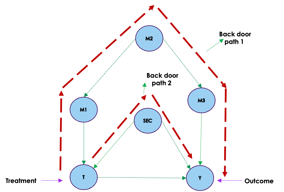
Let us look at the causal graph given above. From the graph we can see two back door paths from the treatment variable to the outcome. These back door paths has the effect of bringing spurious correlations between the treatment and the outcome because of confounding. As we saw in the blog on causal graph and confounding , to eliminate these spurious correlations and to get the real causal effect between the treatment and outcome variable, we need to block the flow of association through these paths. One way to achieve this is through conditioning on the different variables in the back door paths. We saw this phenomenon on the blog on causal graphs. Let us consider the graph represented below which shows the conditioning on M2 and SEC.

We will get the same effect i.e blocking the back door paths if we condition on on M1 & SEC and/or M3 & SEC.

So by blocking the back door paths, we are eliminating all spurious correlations between the treatment and outcome giving us the real causal effects.

To illustrate the concept further, consider the following examples:

Example 1: Student Performance and Study Hours

Suppose we’re exploring the causal link between sleep duration ((X)) and student performance ((Y)) while considering study hours ((Z)) as a potential confounder. It’s conceivable that students who sleep longer might have more time and energy to dedicate to studying, and this extra study time might enhance their performance.

Direct Path: If we disregard confounding, we might hastily conclude that more sleep directly leads to better academic performance. However, the confounding factor of study hours could be influencing both sleep duration and performance.

Back Door Path: In this context, the back door path would involve controlling for study hours ((Z)). By comparing students who put in similar study hours, we can better uncover the genuine causal relationship between sleep duration and performance. This approach helps us mitigate the influence of the potential confounder, study hours, thus providing a clearer picture of the true impact of sleep duration on academic performance.

Example 2: Yoga, Sleep quality and Mental well-being

Let’s consider a scenario where we’re investigating the causal relationship between practicing yoga ((X)) and mental well-being ((Y)), while considering sleep quality ((Z)) as a potential confounder. People who regularly practice yoga might experience improved sleep quality, and sleep quality could also influence their mental well-being.

Direct Path: Without accounting for sleep quality, we might hastily conclude that practicing yoga directly enhances mental well-being. Yet, the presence of sleep quality as a confounder might impact both the decision to practice yoga and mental well-being.

Back Door Path: In this context, the back door path could involve controlling for sleep quality ((Z)). By comparing individuals with similar sleep quality, we can effectively isolate the genuine causal connection between practicing yoga and mental well-being. This approach helps us mitigate the confounding effect of sleep quality, allowing us to assess the true impact of practicing yoga on mental well-being without undue influence.

Importance of Identifying All Back Door Paths:

Identifying and adjusting for all relevant back door paths is crucial in causal analysis because it helps us avoid drawing incorrect conclusions due to confounding. By considering these paths, we can isolate the true causal relationship between variables and gain accurate insights into how changes in one variable affect another. Failure to consider back door paths can lead to biased estimates and incorrect causal interpretations.

Back door path identification is a strategic approach to untangle the complexity of causal relationships in the presence of confounding variables. By adjusting for these paths, we ensure that our conclusions about causality are accurate and reliable, even in the face of hidden influences. Let us now look at what adjusting for back door paths means

Back door adjustment

In the world of understanding cause and effect, things can get tricky when hidden factors, known as confounding variables, cloud our view. This is where the back door criterion comes in. It’s like a guide that helps us untangle the mess and find out what truly causes what. In our earlier example, lets say we want to know if practicing yoga (X) really improves mental well-being (Y). But there’s a sneaky factor: sleep quality (Z). People who practice yoga tends to sleep well. Now, instead of doing interventions, which can be tricky, we can adjust by considering sleep quality. This is back door adjustment. It’s like simulating interventions without actually intervening. By doing this, we uncover the real connection between yoga and health while avoiding the confusion caused by that sneaky factor. So, the back door criterion is like a secret tool that helps us figure out real cause-and-effect relationships, even when things are a bit tangled up.

Mathematically, the back door adjustment brings in “conditioning” to counteract the impact of confounders. For three variables – let’s call them teaching method (X), student performance (Y), and socioeconomic background (Z) – the equation reads:

P(Y∣do(X))=∑_Z​P(Y∣X,Z)⋅P(Z)

Now, let’s put this into a relatable classroom scenario. We’re looking at two teaching methods (Method A and B) used by students of different socioeconomic statuses (Low, Medium, and High SES) to see how they perform. Our dataset captures all this complexity, noting down the teaching method, socioeconomic status, and performance for each student.

Now, let’s use some simple code to apply this equation. In this example, we’ll focus on the back door path when we zero in on students with Low SES. By doing this, we make sure we account for the influence of socioeconomic status, and this helps us uncover the genuine impact of the teaching method on student performance.

# Given data for the student example
data = np.array([
    [0, 0, 1],  # Method A, Low SES, Pass
    [1, 1, 0],  # Method B, High SES, Fail
    [0, 0, 1],  # Method A, Low SES, Pass
    [1, 2, 1],  # Method B, Medium SES, Pass
    [1, 2, 0],  # Method B, Medium SES, Fail
    [0, 1, 0],  # Method A, High SES, Fail
    [1, 1, 1],  # Method B, High SES, Pass
    [0, 2, 1]   # Method A, Medium SES, Pass
])

# Extract columns for easier calculations
X = data[:, 0]  # Teaching method
Y = data[:, 2]  # Student performance
Z = data[:, 1]  # Socioeconomic status

# Calculate the back door path with conditioning for all values of X
p_Y_do_X_values = []
for x_val in np.unique(X):
    print('value of X',x_val)
    p_Y_do_X_proof = 0

    # Step 1: Start with the definition
    for w in np.unique(Z):
        print('value of Z',w)
        # Step 3: Break down P(y | do(t), w)
        
        p_Y_given_t_w = np.nan_to_num(np.sum(Y[(X == x_val) & (Z == w)]) / np.sum((X == x_val) & (Z == w)))
        # Step 4: Substitute into the equation
        p_w_given_do_t = np.nan_to_num(np.mean(Z[X == x_val]) / np.sum(X == x_val))
        # Step 5: Back door criterion
        p_Y_do_X_proof += p_Y_given_t_w * p_w_given_do_t
    p_Y_do_X_values.append(p_Y_do_X_proof)
    
# Print the results for all values of X
for i, x_val in enumerate(np.unique(X)):
    print(f"P(Y | do(X={x_val})) = {p_Y_do_X_values[i]:.4f}")

The purpose of this code is to get an intuitive understanding on what is going on in the equation. Here we have considered a toy data set.Let’s break down the code and its high-level explanation in the context of the back door equation:

Intuitive Explanation:
This code calculates the adjusted probability (P(Y | do(X))) for various values of (X) using the back door path. It iterates over different values of (X) and considers the influence of confounder (Z) to account for potential bias. The back door path approach allows us to adjust for confounding variables and isolate the causal effect of (X) on (Y).
Imagine we’re in a classroom where we’re trying to understand how different teaching methods ((X)) affect student performance ((Y)), while taking into account their socioeconomic status ((Z)) which might act as a confounder. The goal is to adjust for the confounding effect of (Z) on the relationship between (X) and (Y).

1. Looping Over Values of (X): The code iterates over each unique value of (X) (different teaching methods). For each (X) value, it calculates the adjusted probability (P(Y | do(X))) using the back door path equation.
2. Conditioning on (Z) (Confounder): Inside the loop, the code further iterates over each unique value of (Z) (different socioeconomic statuses). It considers each combination of (X) and (Z) to calculate the adjusted probability. This conditioning on (Z) helps us control for its influence.
3. Adjustment using Back Door Path: For each (X) value and (Z) value combination, the code calculates the probability (P(Y | X = x_{\text{val}}, Z = w)), which represents the likelihood of a student passing given a certain teaching method and socioeconomic status.
4. Weighted Sum for Adjustment: The code then calculates (P(w | do(t))) using the mean of (Z) values where (X = x_{\text{val}}). This corresponds to the proportion of students with a specific socioeconomic status in the context of the chosen teaching method.
5. Back Door Adjustment: It multiplies the calculated probabilities of passing ((P(Y | X = x_{\text{val}}, Z = w))) by the corresponding weight ((P(w | do(t)))) and sums up these adjusted probabilities across all (Z) values. This adjustment accounts for the confounding effect of socioeconomic status and isolates the causal effect of the teaching method ((X)) on student performance ((Y)).
6. Output and Interpretation: The adjusted probabilities for each value of (X) are printed. These adjusted probabilities represent the true causal effects of teaching methods on student performance while considering the influence of socioeconomic status.

In this example we have demonstrated how the back door path is operationalized through iteration, conditioning, and weighted adjustment. This process helps us uncover causal relationships by accounting for confounding variables and yielding insights free from biases introduced by hidden factors.

Having seen back door paths and back door adjustments, let us look at what front door adjustment is.

Front Door Adjustments

In the previous section we discussed how back door paths and adjustments can help us unveil causal relationships. However, what if we’re faced with a scenario where we don’t have access to these back door variables? Imagine we have data generated based on a certain causal graph, but we can’t observe one of the crucial back door variables. This means our usual back door adjustments won’t work. In such cases, the front door criterion offers a solution. It’s a bit like taking a different path to get the same result.

Imagine a scenario where we want to understand how a cause, X (let’s say a new teaching method), affects an effect, Y (student performance). It’s plausible that other variables we may not observe directly, like a student’s motivation or background, could influence both the teaching method chosen (X) and student performance (Y). These unobserved variables are essentially the confounders that can muddy our attempts to establish a causal link between X and Y.

Now, suppose we don’t have access to data on these unobserved confounders. In such cases, establishing causality between X and Y becomes challenging because we can’t directly block the confounding paths through these unobserved variables. However, we observe another variable, M (let’s say the student’s engagement level or effort), that is influenced by X and influences Y.

The variable M is called as a mediator and it plays a significant role in getting the causal effect. It acts as an intermediary step that helps us understand the causal effect of X on Y, even when the direct path from X to Y is blocked by unobserved or unobservable variables (the confounders).

Front Door Variable Adjustment:

Front door variable adjustment is a method used to uncover the causal effect of X on Y through the mediator M, even when the direct path between X and Y is blocked by unobserved or unobservable variables. Let us look at the equation of the front door adjustment

P(y|do(X=x))=∑_zP(z|x)∑_x′P(y|x′,z)P(x′)

Now, let’s dissect this equation step by step:

1. Intervention on X: (X = x) represents the value of X when we intervene or change it to a specific value, denoted as (x). For example, if we want to find the probability that Y equals 1 when we intervene and set X to 1: [ P(Y | do(x)) { when Y = 1 and X = 1} ]
2. Values of X before Intervention: (X = x’) represents the values of X before any intervention. This is found within the inner summation. For instance:

• (P(z = 0 | x = 1) * [∑_x′ P(Y = 1 | x’, z = 0) P(x’)] ) This part considers the probability of Z being 0 given X is 1, and then it sums over all possible values of X’ before the intervention. It calculates the contribution to the overall probability of Y = 1 when X is intervened upon.
• Similarly, (P(z = 1 | x = 1) * [∑_x P(Y = 1 | x’, z = 1) P(x’)]) accounts for the probability of Z being 1 given X is 1, and it sums over all possible values of X’ before the intervention.

Now that we have seen the equations, let us break down the equation and provide an interpretation of the process using code. We will give a step by step explanation and relate it to the front door adjustment criteria. To illustrate the front door adjustment criteria, we’ll use a causal scenario involving three variables: X (the treatment), Z (the mediator), and Y (the outcome).

Step 1: Simulating Data

# Simulate the distribution of X before intervention
p_x_before = np.array([0.4, 0.6])  # P(X=x')
x_before = np.random.choice([0, 1], size=n_samples, p=p_x_before)

Here, we start by simulating the distribution of X before any intervention. In this example, we have two possible values for X: 0 and 1. This represents different treatment options.

Step 2: Simulate the distribution of Z given X

# Simulate the distribution of Z given X
p_z_given_x = np.array([[0.7, 0.3], [0.2, 0.8]])  # P(Z=z | X=x')
z_given_x = np.zeros(n_samples)
for i in range(n_samples):
    z_given_x[i] = np.random.choice([0, 1], size=1, p=p_z_given_x[x_before[i]])

Now, we simulate the distribution of Z given X. This represents how the mediator (Z) behaves depending on the treatment (X). We have conditional probabilities here. For example, when X=0, the probabilities for Z=0 and Z=1 are 0.7 and 0.3, respectively.

Step 3: Simulate the distribution of Y given X, Z

# Simulate the distribution of Y given X, Z
p_y_given_xz = np.array([[[0.9, 0.1], [0.2, 0.8]], [[0.6, 0.4], [0.1, 0.9]]])

Here, we simulate the distribution of Y given X and Z. This represents how the outcome (Y) is influenced by both the treatment (X) and the mediator (Z). The nested array structure corresponds to conditional probabilities. For example, when X=0 and Z=0, the probability of Y=1 is 0.9.

Step 4: Normalize the Conditional Probability Distributions

# Normalize the conditional probability distributions
p_y_given_xz_norm = p_y_given_xz / np.sum(p_y_given_xz, axis=2, keepdims=True)

To ensure that our conditional probability distributions sum to 1, we normalize them. This normalization is crucial for accurate calculations.

Step 5: Calculate P(y=1 | do(X=x))

# Calculate P(y=1 | do(X=x))
x_intervention = 1
p_y_do_x = 0

for z_val in [0, 1]:
    p_z_given_x_intervention = p_z_given_x[x_intervention, z_val]
    p_y_given_xz_intervention = p_y_given_xz_norm[x_intervention, z_val, 1]  # P(Y=1 | X=x, Z=z)
    p_x_before_intervention = p_x_before[x_intervention]

    p_y_do_x += p_z_given_x_intervention * p_y_given_xz_intervention * p_x_before_intervention

This is where we apply the front door adjustment criteria. We want to find the probability of Y=1 when we intervene and set X to a specific value (x_intervention). We do this by considering different values of Z (the mediator) and calculating the contribution of each value to the final probability. We use the normalized conditional probability distributions to ensure accurate calculations.

Practical Use Case: Imagine X represents a medical treatment, Z is a biological mediator, and Y is a patient’s health outcome. The code simulates how we can estimate the effect of the treatment (X) on health (Y) while accounting for the mediator (Z). By adjusting for Z, we isolate the direct effect of the treatment, which is essential in medical research to understand treatment efficacy.

In summary, this code demonstrates the front door adjustment criteria by simulating a causal scenario and calculating the causal effect of a treatment variable while considering a mediator variable. It ensures that we account for the mediator’s influence on the outcome when estimating causal effects.

Instrumental Variables :

Imagine you want to know if eating more vegetables makes people healthier. But here’s the issue: people who eat more veggies might also do more exercise, and that exercise could be the real reason they’re healthier. So, there’s a sneaky variable, exercise, that you can’t really measure, but it’s affecting both eating veggies and being healthy.

Instrumental variables are like detective tools in such situations. They’re special variables that you can see and control. You use them to help figure out the real cause.

Here’s how they work: You find an instrumental variable that’s linked to eating veggies (X) but doesn’t directly affect health (Y). It’s like a stand-in for the exercise you can’t measure. Then, you use this instrumental variable to uncover if eating more veggies really makes people healthier.

So, instrumental variables help cut through the confusion caused by hidden factors, letting you discover the true cause-and-effect relationship between things, even when you can’t see all the pieces of the puzzle.

Selection of instrumental variables : Instrumental variables are carefully chosen based on specific criteria. They should exhibit a correlation with the Outcome variable (Y) however, they must not have any direct causal effect on the outcome (Y) apart from their influence on the treatment. This criterion ensures that the IV only affects the outcome through its impact on the treatment, making it a valid instrument.

Causal Effect on the Treatment Variable:One critical characteristic of an instrument variable is that it has a causal effect on the treatment variable (X). This means that changes in the IV lead to changes in X. This causal link is essential because it enables the IV to affect the treatment variable in a way that can be exploited to estimate causal effects.

Random Assignment:An ideal instrumental variable is one that is randomly assigned or naturally occurring in a way that is akin to randomization. This random assignment ensures that the IV is not influenced by any other confounding variables. In other words, the IV should not be correlated with any unobserved or omitted variables that might affect the outcome. Random assignment strengthens the validity of the IV approach and helps in isolating the causal relationship between X and Y.

Let us now generate code to understand the role of instrument variables in causal analysis. We will take an example on education level and higher wages to explain the concept of instrument variables. This example is heavily inspired by the example demonstrated in the attached link.

Let us first define the problem first

In many real-world scenarios, there is a common observation: individuals with higher levels of education tend to earn higher wages. This positive correlation between education and wages suggests that, on average, people with more years of schooling tend to have higher incomes. Let us generate some synthetic data to elucidate this fact and ask some questions on this phenomenon.

import numpy as np
import matplotlib.pyplot as plt

# Set a random seed for reproducibility
np.random.seed(0)

# Generate synthetic data
n_samples = 1000
education_years = np.random.randint(8, 20, n_samples)  # Simulate years of education (e.g., between 8 and 20)
# Simulate hourly wages as a linear function of education with added noise
hourly_wages = 15 * education_years + 10 + np.random.normal(0, 10, n_samples)

# Create a scatter plot to visualize the correlation
plt.figure(figsize=(8, 6))
plt.scatter(education_years, hourly_wages, alpha=0.5)
plt.title('Synthetic Data: Education vs. Hourly Wages')
plt.xlabel('Years of Education')
plt.ylabel('Hourly Wages')
plt.grid(True)

# Add a trendline to visualize the positive correlation
z = np.polyfit(education_years, hourly_wages, 1)
p = np.poly1d(z)
plt.plot(education_years, p(education_years), "r--")

plt.show()

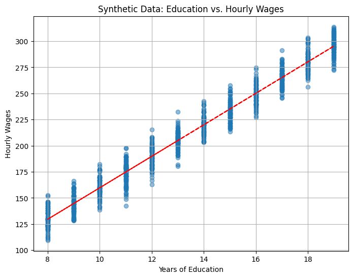
Now, the question arises: Does this positive correlation imply a causal relationship? In other words, does getting more education directly cause individuals to earn higher wages? However, keep in mind that correlation alone does not prove causation. There would be limitations of inferring causality from the correlations between years of education and hourly wages. Here’s an analysis of this specific scenario and our choice of actions

1. Causality Requires Controlled Experiments: To establish a causal relationship between an independent variable (in this case, years of education) and a dependent variable (hourly wages), it’s ideal to conduct controlled experiments. In a controlled experiment, researchers can randomly assign individuals to different levels of education and then observe the impact on wages. Random assignment helps ensure that any observed differences in wages are likely due to the manipulation of the independent variable (education) rather than other confounding factors.
2. Non-Random Assignment in the Real World: However in the real world, we often cannot conduct controlled experiments, especially when it comes to factors like education. Education is typically a choice made by individuals based on various factors such as personal interests, socioeconomic background, career goals, and more. It’s not randomly assigned like it would be in an experiment.
3. Endogeneity and Confounding: When individuals choose their level of education based on their personal circumstances and goals, this introduces the possibility of endogeneity. Endogeneity means that there may be unobserved or omitted variables that influence both education choices and wages. These unobserved variables are the confounders which we have dealt with in depth in other examples. For example, personal motivation, intelligence, or family background could be confounding factors that affect both education choices and earning potential.
4. Correlation vs. Causation: The positive correlation between education and wages simply means that, on average, individuals with more education tend to earn higher wages. However, this correlation does not, by itself, prove causation. It could be that individuals who are naturally more motivated or come from wealthier families are both more likely to pursue higher education and to earn higher wages later in life.

Let us take that the unobserved confounder in our case is the motivation level of induvial. Let us again generate some data to study its relationship with both the treatment ( education ) and outcome ( higher wages )

import numpy as np

import matplotlib.pyplot as plt

# Set a random seed for reproducibility

np.random.seed(0)

# Generate synthetic data for education years and hourly wages (same as before)

n_samples = 1000

education_years = np.random.randint(8, 20, n_samples)  # Simulate years of education (e.g., between 8 and 20)

hourly_wages = 15 * education_years + 10 + np.random.normal(0, 10, n_samples)

# Generate synthetic data for motivation levels

motivation_levels = 0.5 * education_years + 0.3 * hourly_wages + np.random.normal(0, 5, n_samples)

# Create scatter plots to visualize correlations

plt.figure(figsize=(12, 5))

# Education vs. Motivation Levels

plt.subplot(1, 2, 1)

plt.scatter(education_years, motivation_levels, alpha=0.5)

plt.title('Education vs. Motivation Levels')

plt.xlabel('Years of Education')

plt.ylabel('Motivation Levels')

plt.grid(True)

# Hourly Wages vs. Motivation Levels

plt.subplot(1, 2, 2)

plt.scatter(hourly_wages, motivation_levels, alpha=0.5)

plt.title('Hourly Wages vs. Motivation Levels')

plt.xlabel('Hourly Wages')

plt.ylabel('Motivation Levels')

plt.grid(True)

plt.tight_layout()

plt.show()

In this synthetic data, we’ve introduced motivation levels as a function of both education years and hourly wages, with some added random noise. As seen in the scatter plots, there is a positive correlation between motivation levels and both education years and hourly wages. This example is only to illustrate how an unobserved confounder (motivation levels) can influence both the treatment variable (education) and the outcome (hourly wages), potentially leading to a spurious correlation between education and wages.

However we have a problem here. We know that motivation level is a good confounder which will influence both the treatment and outcome. However we cant observe or collect data for a variable like motivation levels. So without getting data on the confounder how to we adjust the confounder to get this true causal effect between the treatment and outcome ? This is where instrumental variables (IVs) come into play.

This is how we will go about this task

1. Identify an Instrument: An instrumental variable (IV) is a variable that has causal relationship with the treatment variable (education) but does not have a direct causal effect on the outcome (hourly wages). The IV should only affect the outcome through its impact on the treatment.
2. Random Assignment: The IV should be assigned randomly or at least exogenously (not influenced by other confounding variables). This ensures that the IV is not subject to the same confounding factors as education.

In practice, finding a suitable instrumental variable can be challenging. It needs to meet the criteria of relevance (correlated with education) and exogeneity (not directly affecting wages). Once an appropriate IV is identified, it can help us estimate the causal effect of education on wages while addressing the issue of unobserved confounders like motivation

A good instrumental variable (IV) in the case of education and higher wages would be a variable that affects a person’s level of education but does not directly affect their wages. This IV should be correlated with education and exogenous, meaning it’s not influenced by the same factors that affect wages. One potential IV in this context is “compulsory schooling laws.”

Here’s how it works:

1. Compulsory Schooling Laws: In some regions or countries, there are laws that require children to stay in school until a certain age or grade level. These laws effectively determine the minimum level of education a person must receive.
2. Relevance: Compulsory schooling laws are relevant because they impact the educational attainment of individuals. People are compelled to stay in school up to a certain level, which influences their years of education.
3. Exogeneity: The decision to implement compulsory schooling laws is typically made by governments and is not influenced by individual motivations, abilities, or job opportunities. Therefore, it can be considered exogenous in the context of individual wage determinants.
4. Causal Effect: Compulsory schooling laws have a causal effect on education because they mandate a minimum level of schooling. However, they do not directly affect wages. The relationship between these laws and wages is mediated through the educational attainment they enforce.

Let us now generate more synthetic data to show the desired effect between instrument variables and other variables.

import numpy as np

import matplotlib.pyplot as plt

# Number of samples

n_samples = 1000

# Generate compulsory schooling levels (IV)

compulsory_schooling = np.random.randint(10, 16, size=n_samples)  # Random values between 10 and 15

# Generate education levels influenced by compulsory schooling

education = compulsory_schooling + np.random.normal(0, 2, size=n_samples)  # Adding some noise

# Generate wages influenced by education

wages = 1000 + 500 * education + np.random.normal(0, 1000, size=n_samples)  # Adding noise

# Generate random motivation levels

motivation = np.random.normal(50, 20, size=n_samples)  # Random normal distribution

# Create subplots

fig, axs = plt.subplots(1, 3, figsize=(18, 5))

# Plot education vs. compulsory schooling

axs[0].plot(compulsory_schooling, education, 'bo', alpha=0.5)

axs[0].set_xlabel("Compulsory Schooling Years")

axs[0].set_ylabel("Education Years")

axs[0].set_title("Positive Correlation: Education vs. Compulsory Schooling")

# Plot wages vs. compulsory schooling

axs[1].plot(compulsory_schooling, wages, 'go', alpha=0.5)

axs[1].set_xlabel("Compulsory Schooling Years")

axs[1].set_ylabel("Hourly Wages")

axs[1].set_title("Positive Correlation: Wages vs. Compulsory Schooling")

# Plot motivation vs. compulsory schooling

axs[2].plot(compulsory_schooling, motivation, 'ro', alpha=0.5)

axs[2].set_xlabel("Compulsory Schooling Years")

axs[2].set_ylabel("Motivation Level")

axs[2].set_title("No Correlation: Motivation vs. Compulsory Schooling")

plt.tight_layout()

plt.show()

From the plots, we can clearly observe the positive correlation between the instrument variable (compulsory schooling) and both the treatment (education) and the outcome (hourly wages). . Furthermore, we know that the instrument (compulsory schooling) has a causal effect on the treatment (education) because it determines the minimum number of years an individual must attend school. This satisfies one of the key conditions for a valid instrument.

Another critical condition for a valid instrument is that it should not be correlated with confounding variables that might distort the causal relationship. In our case, we can see from the plots that there is no apparent correlation between compulsory schooling and motivation levels, which is a good sign. This lack of correlation suggests that our instrument is not influenced by unobserved factors that could confound our analysis.

In summary, these plots demonstrate the significance of using an instrument variable in causal analysis. They illustrate that a well-chosen instrument can exhibit a clear causal effect on the treatment while also having a positive correlation with both the treatment and the outcome. Moreover, the absence of correlation between the instrument and potential confounders enhances the credibility of our causal inferences. Instrumental variables provide a powerful way to disentangle causation from correlation in situations where direct causality is challenging to establish, making them a valuable tool in causal analysis.

Wrapping up

In this exploration of causal inference, we’ve delved into three essential concepts: the back door criterion, the front door criterion, and instrumental variables. The back door criterion serves as our guide in identifying the necessary variables for adjusting causal relationships and helps us uncover the true causal effects in observational data. Meanwhile, the front door criterion reveals an intriguing pathway where we can understand the impact of an exposure on an outcome, even when the direct path is blocked by unobserved variables. Finally, instrumental variables emerge as powerful tools to address endogeneity and establish causality by leveraging variables with known causal effects and correlations with both the treatment and the outcome.

These methods are not merely theoretical constructs; they play a pivotal role in extracting causal insights from real-world data. By diligently following the criteria of these causal inference techniques, researchers can navigate the complex landscape of observational data, disentangle confounding relationships, and ultimately gain a deeper understanding of cause and effect. These tools empower us to make more informed decisions, whether in public health, economics, or any field where causal relationships matter. As we continue to refine these methods and develop new ones, the horizon of causal inference expands, offering us ever more precise insights into the complex web of causality that shapes our world.