

Structure
- Introduction to causal analysis
- Implementation of causal analysis using DoWhy
- Business context – Member loyalty program
- Causal analysis process in a nutshell
- Process 1 : Defining the problem statement
- Process 2 : Data preparation through simulation
- Defining treatment and control for membership program
- Creation of simulated data for causal analysis
- Process 3 : Defining the causal graph structure
- Process 4 : Causal identification
- Identification of back door, front door and instrumental variables
- Conclusion – Processes to be implemented in Part II of the series
Introduction
In this series, we’re introducing a paradigm that’s very important in the world of artificial intelligence, Causal AI. While traditional AI focuses on predicting outcomes based on data patterns, Causal AI delves much deeper. It’s all about understanding the ‘why’ behind those patterns, uncovering the intricate cause-and-effect relationships that govern our world. So, if you’ve ever wondered about the true reasons behind data trends, or if you’re curious about how different variables interact to create real-world impacts, then you’re in for an exciting journey.
Imagine you’re running an online streaming platform, and you’ve noticed that whenever you recommend certain songs to users, they not only listen to those songs but also stay on your platform longer, leading to increased revenue.
Traditional AI would say, “When we recommend these songs, users stay longer, and we earn more.” But Causal AI would take it a step further digging deeper to reveal the underlying cause. It might find that the songs you recommend have a specific beat or rhythm that makes users more engaged. It’s like discovering that the secret ingredient in a recipe is a unique spice and explain, “When we recommend these songs, it causes users to stay longer and explore more music, which directly leads to increased revenue.”

This understanding is incredibly valuable. It means you can not only predict but also influence user behavior. You can fine-tune your recommendations to include songs with similar engaging beats, further enhancing user engagement and revenue.
Causal AI doesn’t just stop at stating an effect; it uncovers the causal chain and reveals the hidden connections between variables. It’s like being a detective in the world of data, solving mysteries and using those insights to drive success in various domains. Causal AI has immense implications for fields like healthcare, economics, social sciences, and beyond.
Causal analysis Implementation – Introducing Do Why
When it comes to learning causal analysis, there are different approaches: diving into the theories and building methods from the ground up, or taking advantage of existing packages and tools. The former option is rich in educational value but can be time-consuming. On the other hand, the latter, using specialized packages, can get the job done quickly but might leave you in the dark about what’s happening beneath the surface. In this series, we’re offering a hybrid approach. We’ll leverage a powerful package, DoWhy, while also taking a deep dive into the underlying theory.
Speaking of packages, there are several exceptional ones available, such as DoWhy, CausalML, CausalImpact, EconML, and more. Our journey into the world of causal analysis begins with DoWhy.
But why DoWhy? The answer is simplicity. DoWhy allows us to conduct complex causal analyses with just a few lines of code, making it a practical choice. However, don’t let this simplicity fool you. Behind each line of code lies a profound theoretical foundation, shaping every aspect of the analysis process.
In this series, we’re pulling back the curtain. We won’t just show you how to execute essential causal analysis steps; we’ll also explore the theories that underpin them. For example, consider the crucial task of identifying causal effects. DoWhy makes it look easy with a single line of code. But beneath that simplicity lies a sequence of steps, including:
- Building a causal graph
- Identifying causal effects
- Ensuring identifiability
- Estimating causal effects
Understanding each of these steps is critical to get an intuitive understanding of what we are attempting to do . In this series we will break down each of the implementation steps into its component processes and then we’ll dissect these process to its core, understanding why we perform each step and how it contributes to our intuitive comprehension of causal relationships. So, join us as we bridge the gap between theory and practice, empowering you to wield the true power of Causal AI.
Problem Statement
As this is an introductory series, we will delve with a simple problem statement. This is taken from the example available in Microsoft research on estimating the effect of a Member Rewards program from the following link. Let us first understand the business context for this problem statement
Business Context – Members loyalty program

In today’s competitive business landscape, companies strive to attract and retain customers by offering various loyalty programs and subscription services. One common question that arises in these scenarios is whether these programs truly have a positive impact on business outcomes. To answer this question, we need to go beyond simple correlation and apply causal analysis techniques. In this blog post, we will explore how causal analysis can help us estimate the effect of a member rewards program on total sales, providing valuable insights for businesses.
Importance of the Problem:
The impact of a member rewards program on total sales is a critical aspect for businesses to evaluate. By understanding the causal relationship between offering such a program and customer spending, companies can make informed decisions about resource allocation, marketing strategies, and program optimization. Answering the question of whether the program is effective allows businesses to measure its return on investment, identify areas for improvement, and enhance customer loyalty.
The problem of estimating the effect of a member rewards program is just one example of many business problems that can be addressed using causal analysis. Consider the following scenarios:
- Pricing Strategy: A company wants to determine the impact of a price change on sales volume. Causal analysis can help isolate the effect of price from other factors and provide insights into optimal pricing strategies.
- Marketing Campaigns: Businesses invest significant resources in marketing campaigns. Causal analysis can help measure the effectiveness of different marketing channels, messages, or promotions, enabling companies to allocate their marketing budget wisely.
- Product Development: When introducing a new product or feature, companies need to assess its impact on customer satisfaction and sales. Causal analysis can uncover the causal relationship between the product and desired outcomes, guiding product development decisions.
Causal Analysis in a Nutshell:
Causal analysis is an analytical approach that aims to understand cause-and-effect relationships between variables. Unlike correlational analysis, which examines associations between variables, causal analysis goes a step further to determine the true causal impact of an intervention or treatment on an outcome of interest. Let us look at all the steps involved in causal analysis. Many of the terms defined in these steps might sound alien at this point of time. However by end of this series you would pretty well understand the nuances of all these terms.

- Problem Statement Definition:
To conduct a meaningful analysis, we define the problem statement and research question clearly. For instance, we pose the question: “What is the causal effect of the membership loyalty program on buying patterns?” Here, the focus is on understanding how the loyalty program influences customers’ buying propensities. - Data Collection and Cleaning:
In order to analyze the impact of a membership loyalty program on customer retention, we begin by collecting and cleaning relevant data. This may include customer profiles, enrollment information, and purchase history. For example, we gather data on the number of months a customer has been a member, their total spendings, and the frequency of their purchases. - Causal Graph Specification:
Constructing a causal graph allows us to visually represent the hypothesized causal relationships among variables in the membership loyalty program. Consider variables such as enrollment in the program, customer demographics, purchase behavior, and retention rates. For example, the graph may show that program enrollment affects customer satisfaction, which in turn influences their likelihood of remaining loyal to the brand. By specifying the causal graph, we aim to capture the potential causal pathways and identify confounding variables. - Identification of Causal Effect:
Identifying the causal effect involves determining the variables that need to be controlled for to estimate the impact of the loyalty program accurately. For instance, we identify potential confounders that could bias the estimation, such as age, income, or previous purchase frequency, which may affect both enrollment in the program and customer retention. The objective is to identify and account for the variables that could influence the causal relationship between the loyalty program and customer retention. - Selection of Estimation Method:
Based on the data characteristics and assumptions made in the causal graph, we select an appropriate estimation method. For example, we may choose propensity score matching, logistic regression with covariate adjustment, or survival analysis. The selected method should address confounding variables and provide reliable estimates of the causal effect. The objective is to choose a statistical technique that best suits the data and assumptions to estimate the impact accurately. - Estimation of Causal Effect:
Using the chosen estimation method, we estimate the causal effect of the membership loyalty program on customer retention. By running the statistical analysis and adjusting for confounding variables, we quantify the impact of the program. For example, we may find that customers who participate in the loyalty program have a 20% higher likelihood of remaining loyal compared to non-participants. The objective is to obtain a quantitative measure of the program’s impact on customer retention and assess its statistical significance. - Sensitivity Analysis:
To test the robustness of the estimated causal effect, we conduct sensitivity analyses. This involves exploring the sensitivity of the results to different model specifications, inclusion/exclusion of variables, or alternative estimation techniques. For example, we may vary the set of confounding variables or use different statistical models to assess the stability of the estimated effect. The objective is to evaluate the robustness of the findings and ensure that the estimated causal effect is not overly sensitive to modeling choices.
By applying causal analysis techniques, businesses can move beyond mere observations and correlations, gaining deeper insights into the drivers of business outcomes. This empowers decision-makers to make evidence-based choices, optimize strategies, and maximize their competitive advantage. So, let’s roll up our sleeves, delve into the exciting world of causal analysis . Together, we’ll uncover the story behind customer behaviors, the impact of our membership rewards program, and the strategies that will drive our business success.
Process 1 : Defining the problem statement
In causal analysis, it is crucial to define the problem statement and research question clearly to conduct a meaningful analysis. In the context of the membership loyalty program, we can define the problem statement as follows:
“What is the causal effect of the membership loyalty program on buying patterns?”
This problem statement aims to investigate the impact of the loyalty program on customers’ purchasing behaviors and understand whether the program has a positive influence on their buying propensities.
Alongside the problem statement, we can also define the counterfactual question:
“If customers had not enrolled in the membership loyalty program, how would their buying patterns differ?”
This counterfactual question explores the hypothetical scenario where customers did not participate in the program and seeks to determine the difference in their purchasing behaviors compared to the observed scenario.
Causal analysis processes, such as data preparation, causal graph specification, identification, estimation, and refutation, are aligned with providing answers to these questions. The data preparation stage involves cleaning and transforming the data to facilitate the analysis of the loyalty program’s effect on buying patterns. The specification of a causal graph helps identify the variables and their relationships relevant to the research question. The identification step determines whether the causal effect can be estimated given the available data and assumptions. Estimation techniques are then applied to estimate the actual causal effect. Finally, refutation methods are used to test the robustness and sensitivity of the causal model to different assumptions and specifications.
Next, let us now prepare the data required for our analysis.
Process 2 : Data preparation through simulation
Let’s embark on our journey of causal analysis by creating a simulated dataset for our problem statement. Imagine we have a bustling online platform with 10,000 customers, each with their unique preferences and behaviors. Some of these customers have eagerly signed up for our membership rewards program, while others have chosen not to participate. To add some excitement, let’s assign each signing-up customer a specific month when they joined the program, ranging from January to December.
import numpy as np
# Defining the users and the number of months
num_users = 10000
num_months = 12
# Random generation of sign up months
signup_months = np.random.choice(np.arange(1, num_months), num_users) * np.random.randint(0,2, size=num_users)
The code snippet provided generates a simulated dataset for the problem statement. Let’s break it down step by step:
num_users = 10000: This line sets the number of users in our dataset to 10,000. Each user represents a customer on our online platform.num_months = 12: This line sets the number of months we want to simulate in our dataset. In this case, we have 12 months, representing a year.signup_months = np.random.choice(np.arange(1, num_months), num_users) * np.random.randint(0, 2, size=num_users): This line generates random signup months for the users in our dataset. Let’s break it down further:
np.arange(1, num_months): This generates an array containing numbers from 1 tonum_months - 1, representing the available signup months from January to Decembernp.random.choice(...): This function randomly selects signup months for each user from the array generated in the previous step. Thenum_usersparameter specifies the number of choices to make.np.random.randint(0, 2, size=num_users): This generates an array of random 0s and 1s, representing whether a user has signed up (1) or not (0). Thesizeparameter specifies the size of the array.- This performs element-wise multiplication between the two arrays. As a result, users who have not signed up (0) will have a signup month of 0, and users who have signed up (1) will have a randomly assigned signup month.
Creating this dataset allows us to explore the impact of our membership rewards program on total sales and delve into the realm of causal analysis. By simulating customer behaviors, we can examine how different factors, such as program participation and signup month, influence customer spending patterns. Through this process, we can unravel the causal relationships that drive our business outcomes and gain valuable insights for decision-making.
To conduct our analysis on the membership program, we create a dataframe that contains the necessary data. The dataframe, named ‘df’, includes the following information:
- User ID: Each unique user is assigned a unique ID ranging from 1 to 10,000. This allows us to identify and track individual users throughout the analysis.
- Signup Month: This column indicates the month in which a specific user signed up for the membership program. The signup month is represented by a number between 1 and 12. A value of 0 indicates that the user has not signed up for the program. For example, a user with a signup month of 3 indicates they joined the program in March.
- Month: This column represents the months of the year, ranging from 1 to 12. It indicates the time period for which we have data on customer purchases and program participation.
- Purchase Presence: This feature indicates whether a customer made a purchase in a particular month. It is designed in a way that ensures every customer has a presence in each month of the year. For instance, a value of 1 indicates that the customer made a purchase during that month, while a value of 0 indicates no purchase.
- Spend: This column represents the aggregated purchase amount for each customer in a given month. The values are randomly generated based on a Poisson distribution with a mean of 500. This simulates the varying spending patterns of customers throughout the year.
The code snippet used to create the dataframe is as follows:
df = pd.DataFrame({
    'user_id': np.repeat(np.arange(num_users), num_months),
    'signup_month': np.repeat(signup_months, num_months),
    'month': np.tile(np.arange(1, num_months+1), num_users),
    'spend': np.random.poisson(500, num_users*num_months)
})
In this code, we utilize the np.repeat() function to repeat the values of user_id and signup_month for each month, ensuring that each user has an entry for every month in the dataframe. Similarly, the np.tile() function is used to replicate the sequence of months for each user. Lastly, the np.random.poisson() function generates random purchase amounts based on a Poisson distribution with a mean of 500.
The resulting dataframe df provides the necessary data to analyze the impact of the membership program on customer purchasing behavior. It allows us to examine the relationship between signup months, customer purchases, and spending patterns over time. Now that we have simulated the basic data set, let us introduce some important concepts of causal analysis i.e treatment group and control groups.
Defining treatment and control for membership program
In causal analysis, two essential concepts that play a vital role in evaluating the impact of a membership program are the treatment group and the control group. These groups are integral to understanding the causal effects of the program on customer behavior and outcomes. To know more about treatment group and control group you can refer to this link.
The treatment group in the context of our membership program refers to customers who have actively signed up and participated in the program. These individuals have voluntarily chosen to engage with the program and are exposed to the additional benefits, rewards, and experiences offered. By being part of the treatment group, these customers potentially experience a different set of circumstances compared to the control group.
On the other hand, the control group consists of customers who have not signed up for the membership program. They represent a baseline or reference group that reflects what would happen in the absence of the program. These customers do not receive the program’s benefits, rewards, or any specific treatment related to membership. The control group provides a comparison point to evaluate the impact of the program by serving as a counterfactual scenario.
By distinguishing between the treatment and control groups, we can assess the causal effect of the membership program on various outcomes, such as customer spending, engagement, loyalty, or any other relevant metrics. Understanding the distinct characteristics and behaviors of both the treatment and control groups enables us to explore questions such as:
- How does customer spending differ between those who signed up for the program and those who did not?
- What is the incremental impact of the program on customer retention or lifetime value?
Answering these questions requires careful analysis of the treatment and control groups, allowing us to draw valid causal inferences and make informed decisions regarding the membership program’s efficacy and potential optimization.
Having understood about treatment group and control group let us define them in our data set.
The above code manipulates the data frame to simulate the treatment effect and generate data for the treatment and control groups.
# A customer is in the treatment group if and only if they signed up
df["treatment"] = df["signup_month"]>0
# Simulating an effect of month (monotonically decreasing--customers buy less later in the year)
df["spend"] = df["spend"] - df["month"]*10
# Simulating a simple treatment effect of 100
after_signup = (df["signup_month"] < df["month"]) & (df["treatment"])
df.loc[after_signup,"spend"] = df[after_signup]["spend"] + 100
df

Let us understand the processes which we have implemented in the code block above to simulate the data for our analysis.
- Defining the Treatment Group: The line
df["treatment"] = df["signup_month"]>0creates a new column named “treatment” in the data frame. A customer is assigned to the treatment group if their “signup_month” is greater than zero, indicating that they have signed up for the membership program. This step distinguishes between the customers who have actively engaged with the program (treatment group) and those who have not (control group). - Simulating the Effect of Time: The line
df["spend"] = df["spend"] - df["month"]*10simulates a time-related effect on customer spending. It reduces the “spend” values based on the corresponding “month” values in a monotonically decreasing manner. This simulation implies that customers tend to spend less as the year progresses. - Simulating a Treatment Effect: The line
after_signup = (df["signup_month"] < df["month"]) & (df["treatment"])creates a Boolean mask to identify the customers who signed up before the current month (indicating they are eligible for the treatment) and are still in the treatment group. This condition represents the period after customers have signed up but are still active members of the program. - Applying the Treatment Effect: The line
df.loc[after_signup,"spend"] = df[after_signup]["spend"] + 100modifies the “spend” values for the customers who meet the condition defined by the “after_signup” mask. It adds a treatment effect of 100 to their spending, representing an increase in spending as a result of being part of the membership program.
By applying these simulations, the code generates a data frame that reflects the characteristics of the treatment and control groups. It incorporates the impact of time on customer spending and introduces a specific treatment effect for the customers who signed up and are still active members. This data frame allows for further analysis and estimation of the causal effect of the membership program on customer spending.
Process 3 : Defining the causal graph structure
In the context of causal analysis, constructing a causal graph is a fundamental step as it allows us to visually and systematically represent the relationships between variables within a causal system. A causal graph serves as a graphical depiction of the causal connections between variables, with directed edges indicating the direction of causation. When creating a causal graph, it is essential to have a deep understanding of the domain under study, as the structure of the graph should accurately reflect the true causal relationships that exist within that domain. By incorporating domain knowledge into the construction of the causal graph, we can ensure that the variables and their relationships depicted align with our understanding of how they influence one another in the real-world context. Ultimately, a well-designed causal graph provides a clear and organized representation of the causal structure, facilitating subsequent steps in the causal analysis process. To understand different types of causal graphs and its effect on causal analysis you can refer the following link.
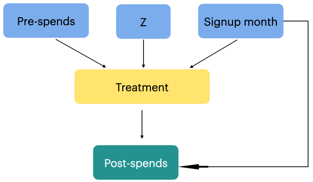
In our problem statement, the outcome which we are trying to understand is whether there is any change in the spending pattern after the sign up month. To do this we need to get the average monthly spending before the signup month and after the signup month. The signup month is an important variable, which in our case is the treatment. For the purpose of our analysis, we take any random month as the signup month, lets say month = 3. The average spending from month 1 to month 2 will be treated as a new variable ‘pre-spends’ and the average spending from month 4 – 11 will be post spends. Often its the buying experiences in the pre-spending period which influences the decision to join the membership program. Once a customer has signed up for the membership program, that decision will influence the post-spending also. So from a causal analysis, the relationship can be represented as follows.

Another important causal relationship to consider is the connection between the signup months and the treatment group assignment. The signup month variable directly influences whether a customer is categorized as part of the treatment group or not. For example, if a customer signs up in month 3, they are included in the treatment group. Additionally, the signup month has a direct relationship with post-spends, as it is associated with seasonal factors that can impact customer spending behavior. For instance, customers who sign up during holiday months might exhibit different post-spending patterns compared to those who sign up during non-holiday months. Understanding and exploring these relationships within a causal analysis framework can provide valuable insights into the effects of signup months on the treatment assignment and subsequent spending behaviour.

In the context of the above causal graph, we need to introduce a new concept called confounding. In causal analysis, a confounder refers to a variable that is associated with both the treatment variable and the outcome variable. It confounds the relationship between the treatment and the outcome because it may independently influence the outcome, creating a spurious association. Confounding variables can lead to biased estimates of the causal effect if not properly accounted for in the analysis.
In this case, the signup month can be considered a confounder. It is associated with both the treatment variable (membership program signup) and the outcome variable (post-spends). The signup month may influence the outcome through its relationship with seasonality and other factors that affect customer spending patterns.
Apart from the signup month, there may be other confounding variables that could impact both the treatment and the outcome. These confounders might include factors such as:
- Customer demographics: Variables like age, gender, income level, or occupation can influence both the decision to sign up for the membership program and post-spending behavior. For example, customers in higher income brackets may be more likely to join the program and spend more.
- Purchase history: The customers’ past purchasing behavior, including the frequency and value of purchases, can be a confounder. Customers who are frequent purchasers or who have a history of high-value purchases may exhibit different spending patterns after signing up for the membership program.
- Geographic location: The geographical location of customers may affect both their likelihood of signing up and their spending patterns. Customers from different regions may have different preferences, access to stores or products, or be influenced by local economic factors.
It is important to note that there may also be unobserved or unidentified confounders that could impact the relationship between the treatment and the outcome. These are confounding variables that are not included in the available dataset or are unknown. Unidentified confounders can introduce bias into the causal analysis and affect the accuracy of the estimated causal effects. Researchers must carefully consider and address both identified and unidentified confounders to obtain reliable causal estimates in their analysis. Please refer to the attached link to know more about confounders
Although we have identified some variables that have a direct influence on the treatment and outcome variables ( confounders ) , it is important to acknowledge that there may be other variables that impact the treatment variable but do not directly affect the outcome variable. Examples of such variables could include the type of products purchased, the length of a user’s account, or the geographic location of the customer. Since we may not have access to all these variables or they may not be directly measurable, we introduce a new variable called an instrumental variable, denoted as ‘z’, in causal analysis. An instrumental variable is a variable that is causally related to the independent variable of interest (treatment) but is not causally related to the outcome variable (post-spends). It helps address potential omitted variable bias and improves the validity of causal inference by isolating the causal effect of the treatment on the outcome.
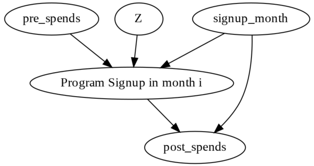
Let us now take into account all these relationships and then represent the final causal graph for this problem statement.
In this causal graph “Z” is the instrumental variable that is causally related to Treatment (“Program Signup in month i ) but not causally related to “post_spends” (the outcome variable). To know more about instrument variables, you can refer the attached link.
To carry on with our causal analysis, which is about identifying whether the membership program had any effect or not, we need to transform the dataset and extract the relevant data. Let’s consider the example of a customer who signed up in the 3rd month. To do this, we modify the data frame by filtering out the customers who either did not sign up (signup_month = 0) or signed up in the 3rd month (signup_month = 3).
# Defining the signup month
i = 3
# Creation of the data frame for customers who have signed up for 4th month

df_i_signupmonth = (
    df[df.signup_month.isin([0, i])]
    .groupby(["user_id", "signup_month", "treatment"])
    .apply(
        lambda x: pd.Series(
            {
                "pre_spends": x.loc[x.month < i, "spend"].mean(),
                "post_spends": x.loc[x.month > i, "spend"].mean(),
            }
        )
    )
    .reset_index()
)
The code snippet performs the following steps:
- We define the signup month of interest as ‘i’, which is set to 3 (representing the 3rd month).
- We create a new data frame, ‘df_i_signupmonth’, by selecting the rows from the original data frame where the signup month is either 0 (indicating no signup) or ‘i’ (the month of interest).
- Next, we group the data frame by ‘user_id’, ‘signup_month’, and ‘treatment’.
- Using the ‘apply’ function, we calculate the average pre-spending and post-spending for each customer who falls into the specified signup month category. The pre_spends are computed by taking the mean of ‘spend’ for the months before the signup month (i.e., where ‘month’ < i), and the post_spends are computed by taking the mean of ‘spend’ for the months after the signup month (i.e., where ‘month’ > i).
- Finally, we reset the index of the data frame to have a clean and organized structure.
The resulting ‘df_i_signupmonth’ data frame contains the pre_spends and post_spends for each customer who signed up in the 3rd month (or did not sign up at all). This transformed dataset allows us to analyze the average treatment effect for customers in the specified signup month, providing insights into how the membership program influenced their spending patterns.
The data frame after these transformation will look as below.

The created data frame, ‘df_i_signupmonth’, is structured in a way that enables further causal analysis. It contains the average spends before and after the signup month for each customer, allowing us to examine the causal effects of the membership program.
Implementation the above processes in Do-why
Now that we have seen some of the initial processes, let us try implementing them using the do-why package. This package can be pip installed as follows.
!pip install dowhy
!pip install EconML
Once the package is installed, we import the package and initialise the causal graph as follows
import dowhy
# Define the causal graph object
causal_graph = """digraph {
treatment[label="Program Signup in month i"];
pre_spends;
post_spends;
Z->treatment;
pre_spends -> treatment;
treatment->post_spends;
signup_month->post_spends;
signup_month->treatment;
}"""
This code defines a causal graph using the DOT language. It models the relationship between treatment (program signup in month i), pre_spends, post_spends, Z (unobserved confounder), and signup_month. Arrows indicate causal connections. This graph suggests that Z affects both treatment and pre_spends, treatment affects post_spends, and signup_month influences treatment and post_spends. This graph is used in DoWhy to identify and estimate causal effects in the presence of unobserved confounding (Z).
Now that we have defined the causal graph and implemented that in do-why, let us analyse the causal path and identify all the components required for causal analysis
Process 4 : Causal Identification
Causal identification refers to the process of determining whether a causal relationship can be inferred between a treatment or intervention and an outcome variable of interest. It involves establishing a causal link by identifying the effect of a specific cause (treatment) on a specific effect (outcome) while considering and controlling for potential confounding factors.
Identifying the causal effect is a critical step in conducting a causal analysis of a membership program. The objective is to determine the impact of the program on customer behavior, specifically their spending patterns. To identify the causal effect, we need to carefully consider the relationship between the treatment variable (program signup in a particular month) and the outcome variable of interest (average post-spends after signup), while accounting for potential confounding factors.
For example, let’s consider a scenario where the membership program offers exclusive discounts and promotions to customers who sign up during holiday months. If we only compare the average post-spends of customers who signed up during holiday months with those who did not sign up, we may mistakenly attribute any differences solely to the program. However, the observed differences could be influenced by other factors such as increased holiday spending trends.
To address this, we need to identify and control for potential confounding variables that could affect both the treatment and the outcome variable. In this case, factors like customers’ purchasing habits prior to signing up for the program, their demographics, or seasonal effects on spending patterns could act as confounders. By including these variables in our analysis and accounting for their influence, we can more accurately isolate the causal effect of the membership program on post-spends.
Causal identification involves the following.
- Identification of backdoor variables: Backdoor variables are variables that are common causes of both the treatment and the outcome. They create confounding bias and can distort the estimated treatment effect if not properly accounted for. Identifying and adjusting for backdoor variables is crucial in establishing a causal relationship between the treatment and outcome. To know more about back door variables and its effects, please refer to this link.
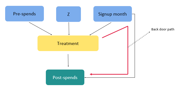
In our context we have only one back door path as shown below.
| Variable | Relationship Characteristics |
| Signup-Month | Back Door Variable |
| Fork type Connection | |
| Conditioning required on the variable to adjust for the effect on outcome |
The only back door path we have is the path from treatment > Sign up month > post spends. This causal path involves a fork type of association and therefore to get an unbiased estimate of the effect of the treatment on the outcome we need to condition on the variable sign up month. We will address these in a little while from now.
- Identification of front door path: Front door variables are variables that lie along the causal pathway between the treatment and outcome, affecting the relationship between them. They are essential for estimating the total causal effect when there are unmeasured confounders or when the treatment-outcome relationship cannot be directly estimated. To know more about front door variables and its importance in causal analysis you can refer this link.
For our problem statement of membership program, we don’t have any front door path as seen from the figure above.
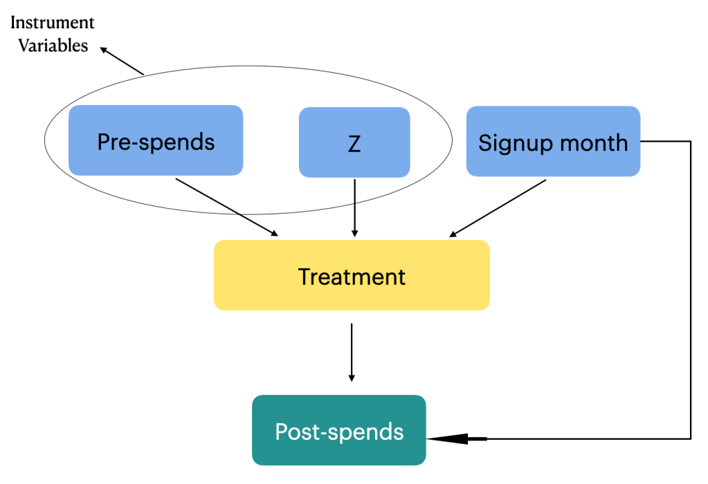
- Identification of instrumental variables: Instrumental variables are variables that are causally related to the treatment but not directly related to the outcome. They are used in situations where there are unobserved confounders or measurement errors. Instrumental variables help to identify the causal effect of the treatment by exploiting their relationship with the treatment variable. You can learn more about instrument variables from this post
We have two instrument variables for our problem statement as seen in the figure below.
By carefully considering backdoor variables, instrumental variables and front door variables causal path analysis allows for a more comprehensive understanding of the causal relationships between the treatment and outcome variables. It helps to mitigate confounding biases, identify indirect effects, and provide insights into the underlying causal mechanisms at play.
Next we will implement these in do-why
# Initialising the causal model
model = dowhy.CausalModel(data=df_i_signupmonth,
                     graph=causal_graph.replace("\n", " "),
                     treatment="treatment",
                     outcome="post_spends")
# Visualising the model
model.view_model()
from IPython.display import Image, display
display(Image(filename="causal_model.png"))
In this code snippet using DoWhy:
- Data Specification:
data=df_i_signupmonthspecifies the dataset (df_i_signupmonth) containing relevant variables. - Graph Specification:
graph=causal_graph.replace("\n", " ")provides the causal graph in DOT format, specifying the relationships between variables. - CausalModel Initialization:
dowhy.CausalModel(...)initializes a causal model.
treatment="treatment"indicates the treatment variable.outcome="post_spends"specifies the outcome variable.
This sets up the structure for causal analysis in DoWhy. The causal graph is crucial for identifying and estimating causal effects, and the treatment and outcome variables are essential components for conducting causal inference.
Having identified the causal relationship, the next task is to get into the important area of causal estimation. We will discuss about the causal estimation and the rest of the process in the second part of the series. Before we sign off on this first part, let us summarise our learning so far.
Wrapping up
In the initial segment of our exploration into causal analysis, we embarked on a journey unraveling the intricacies of causality. Beginning with a comprehensive introduction to the essence of causation, we delved into the significance of the problem statement and the crucial role of the DoWhy package in this domain. The process kicked off with the generation of synthetic data, followed by the critical task of specifying a causal graph. The focal point then shifted to the identification of causal effects, laying the foundation for the second part of our series.
In the second part of the series, we will navigate through the nuanced terrain of selecting estimation methods, a pivotal step in the causal analysis workflow. The journey continues with the estimation of causal effects, exploring the intricacies of propensity score estimation and culminating in the calculation of the Average Treatment Effect (ATE). The DoWhy package will serve as our guiding compass, enabling a practical implementation of these concepts. As we unravel these layers, a holistic understanding of causal analysis will emerge, bridging the theoretical with the practical to empower a deeper grasp of this fascinating field.
