Structure

1. Treatment and Control group in causality
2. Assignment of individuals to treatment and control groups
3. Role of randomization in selection of treatment and control groups
4. Covariates and balancing covariates for treatment and control group
5. Python code exercises on covariate balancing
6. Conclusion

Introduction

Causal analysis is a powerful tool that finds its applications in diverse fields like healthcare, social sciences, and business. It’s the key to unlocking the secrets of cause-and-effect relationships, empowering us to make well-informed decisions. In this exciting journey through causal analysis, our first stop is to dive deep into the world of treatment and control groups. These groups are the building blocks of estimating causal effects, and we’re about to uncover their vital role.

Treatment and Control Group

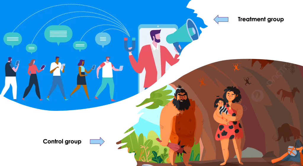
In causal analysis, a treatment group consists of individuals who receive a particular intervention. In contrast, a control group consists of individuals or subjects who do not receive the intervention being studied.Let us look at an example.

Consider a marketing campaign aimed at increasing customer engagement on a company’s website. The treatment group would be the customers who are exposed to the campaign, while the control group would be customers who are not exposed to any promotional activities. By comparing the website engagement metrics between the treatment group and the control group, marketers can assess the effectiveness of the campaign in driving customer engagement.

Let us consider another example in the healthcare domain. Imagine a clinical trial studying the effectiveness of a new drug for treating a certain medical condition. The treatment group consists of participants who receive the new drug, while the control group comprises participants who receive a placebo or standard treatment. By comparing the outcomes between the treatment group and the control group, researchers can determine whether the new drug has a significant impact on improving the condition.

By carefully designing and analyzing studies using these groups, researchers can draw reliable conclusions about the impact of the treatment on the outcome variable. Treatment groups and control groups are essential components of causal analysis for several reasons:

1. Establishing Causality: By comparing the outcomes of the treatment group and control group, helps establish a cause-and-effect relationship
2. Minimizing Bias: The use of control groups helps minimize bias and confounding in the estimation of the causal effect. By ensuring that the only difference between the treatment and control groups is the presence or absence of the treatment, researchers can attribute any observed differences in outcomes to the treatment itself, rather than other factors that may influence the outcome.
3. Counterfactual Analysis: Control groups enables creation of counterfactual scenario, representing what would have happened to the treatment group had they not received the treatment. By comparing the actual outcomes of the treatment group with the hypothetical outcomes of the control group, researchers can estimate the causal effect of the treatment.

Assignment of individuals to treatment or control groups

Individuals are assigned to the treatment group or control group through a process called randomization. Randomization involves randomly assigning individuals to either group, ensuring that each individual has an equal chance of being assigned to either group. This helps minimize bias and ensures that the groups are comparable.

Here are some examples illustrating treatment group and control group in different scenarios:

1. Clinical Trials: In a clinical trial for testing a new drug, participants are randomly assigned to either the treatment group, where they receive the experimental drug, or the control group, where they receive a placebo or standard treatment. The treatment group is used to assess the effectiveness of the new drug compared to the control group.
2. Education Interventions: In an educational study investigating the impact of a teaching method on student performance, students in the treatment group might receive the new teaching method, while those in the control group receive the traditional teaching method. The treatment group is used to evaluate the effectiveness of the new teaching method.
3. Marketing Campaigns: In a marketing study evaluating the effectiveness of a promotional campaign, customers might be divided into a treatment group, exposed to the campaign, and a control group, not exposed to the campaign. The treatment group helps assess the impact of the campaign on customer behavior compared to the control group.

Having see the mechanism of assigning individuals to either groups let us explore the role of randomization in the whole exercise.

Role of randomization in selection of treatment and control groups

Randomization plays a crucial role in assigning individuals to treatment and control groups in causal analysis. It is a fundamental principle that helps ensure the validity and reliability of the findings. By randomly assigning individuals to groups, we introduce an element of chance that reduces the potential for biases that may creep up.

Consider a clinical trial investigating the efficacy of a new drug. Randomization ensures that participants have an equal chance of being assigned to either the treatment group receiving the drug or the control group receiving a placebo ( standard treatment ). Randomization will help avoid selection bias like for instance, individuals with higher risk levels are assigned to the treatment group. As you know individuals with higher risk also can have higher adverse outcomes. This will make these two groups less comparable as one group contains individuals with higher risk factor than the other. So any of the outcomes because of this will be more attributed to the risk factor than the efficacy of the treatment. This is where randomization comes into play. By the process of randomization an individual with a certain risk factor has the chance of being assigned to either of these groups making the groups more comparable.

Covariates and balancing covariates for treatment and control group

Another important factor to consider when assigning individuals into treatment and control group is the influence of covariates. Covariates refer to additional variables or factors that may influence both the assignment of individuals to the treatment or control group and the outcome of interest.

For example in a clinical trial, covariates like age, gender, ethnicity, and medical history can influence both the assignment to treatment groups and the treatment outcomes. For example, older age or the presence of specific medical conditions may affect how individuals respond to the drug or experience side effects. To ensure a fair comparison between treatment and control groups, it is important to consider these covariates. By comparing individuals with similar covariate values across the treatment and control groups, researchers can create balanced comparisons. For instance, comparing the outcomes of individuals aged 50-60 in both groups allows for a more balanced comparison, as it takes into account the potential influence of age on the outcome. On the other hand, comparing individuals aged 50-60 in the treatment group with individuals aged 20-30 in the control group would not provide a balanced comparison, as age is not adequately controlled for. By balancing the covariates, researchers can make more accurate inferences about the treatment effect and minimize the potential confounding effects of covariates on the outcome.

Let us look at a sample code, which attempts to explain the concept of covariate balancing through randomization

import numpy as np
import matplotlib.pyplot as plt

# Generate synthetic data
np.random.seed(0)

# Sample data for Age and Medical History before randomization
age_before = np.random.normal(45, 10, 200)
med_history_before = np.random.choice([0, 1], size=200, p=[0.7, 0.3])

# Sample data for Age and Medical History after randomization
age_after = np.random.normal(50, 8, 200)
med_history_after = np.random.choice([0, 1], size=200, p=[0.5, 0.5])


# Create subplots
fig, axes = plt.subplots(2, 2, figsize=(12, 10))

# Plot Age before and after randomization
axes[0, 0].hist(age_before, bins=20, alpha=0.6, color='blue', label='Before Randomization')
axes[0, 0].set_title('Age Distribution Before Randomization')
axes[0, 0].legend()

axes[0, 1].hist(age_after, bins=20, alpha=0.6, color='red', label='After Randomization')
axes[0, 1].set_title('Age Distribution After Randomization')
axes[0, 1].legend()

# Plot Medical History before and after randomization
axes[1, 0].hist(med_history_before, bins=[-0.5, 0.5, 1.5], rwidth=0.8, alpha=0.6, color='blue', label='Before Randomization')
axes[1, 0].set_title('Medical History Distribution Before Randomization')
axes[1, 0].set_xlabel('Medical History (0: No, 1: Yes)')
axes[1, 0].set_ylabel('Frequency')
axes[1, 0].set_xticks([0, 1])
axes[1, 0].legend()

axes[1, 1].hist(med_history_after, bins=[-0.5, 0.5, 1.5], rwidth=0.8, alpha=0.6, color='red', label='After Randomization')
axes[1, 1].set_title('Medical History Distribution After Randomization')
axes[1, 1].set_xlabel('Medical History (0: No, 1: Yes)')
axes[1, 1].set_ylabel('Frequency')
axes[1, 1].set_xticks([0, 1])
axes[1, 1].legend()

plt.tight_layout()
plt.show()

Let us explain this exercise and provide an intuitive understanding. In the context of randomized experiments, balancing covariates means ensuring that the distribution of certain variables (covariates) is similar or “balanced” between the treatment and control groups. This balance is crucial because it helps eliminate or reduce the potential influence of these covariates on the outcome, allowing researchers to make more accurate inferences about the treatment effect.

In the provided exercise with histograms, we’re examining two hypothetical covariates: Age and Medical History. Here’s how it connects to the concept of balancing covariates:

1. Visualizing Covariate Distributions Before Randomization:

• In the first histogram (Age Distribution), we see the distribution of ages in both the treatment and control groups before randomization.
• Before randomization, the age distributions in the treatment and control groups may be quite different. This lack of balance means that the average age in one group could be significantly different from the other.

1. Visualizing Covariate Distributions After Randomization:

• In the second histogram (Medical History Distribution), we see the distribution of medical history (a binary covariate) in both groups before and after randomization.
• After randomization, the distributions of medical history in the treatment and control groups should ideally be more balanced. This balance suggests that roughly equal proportions of individuals with and without a medical history condition are present in both groups.

The exercise relates to the concept of balancing covariates in the following ways:

• Before Randomization: If covariates like age or medical history are imbalanced between treatment and control groups before randomization, it could lead to confounding effects. For example, if the treatment group has significantly older participants, any observed differences in the outcome may be due to age rather than the treatment itself.
• After Randomization: The goal of randomization is to create groups that are comparable in terms of observed and unobserved covariates. After randomization, we hope to achieve balance in covariate distributions. This balance allows us to attribute any observed differences in outcomes between groups more confidently to the treatment, rather than to covariates.

This exercise illustrates the importance of ensuring covariate balance between treatment and control groups. Achieving this balance through randomization is a fundamental principle of experimental design, as it helps us isolate the true effect of the treatment variable while minimizing the impact of other covariates.

Another way of balancing based on covariates is stratification. Stratification involves dividing the population into strata based on specific covariate values and then randomly assigning individuals from each stratum to the treatment and control groups. This ensures that the groups are balanced within each stratum, even if there are differences across strata. For example, in a study examining the impact of a fitness program on weight loss, participants can be stratified by initial body mass index (BMI) categories, and within each category, individuals are randomly assigned to the treatment or control group. This helps control for the potential effect of the covariate BMI on the outcome. Let us look at an exercise where we achive stratification

import numpy as np
import matplotlib.pyplot as plt
import seaborn as sns

# Simulated data
np.random.seed(0)
n_samples = 200

# Generate age data
age = np.random.choice(['18-30', '31-45', '46-60', '61+'], size=n_samples)

# Create a function to simulate blood pressure based on age and treatment
def simulate_blood_pressure(age, treatment):
    base_pressure = {'18-30': 120, '31-45': 130, '46-60': 140, '61+': 150}
    treatment_effect = {'Treatment': -10, 'Control': 0}
    return base_pressure[age] + treatment_effect[treatment] + np.random.normal(0, 5)

# Create a DataFrame to store the data
import pandas as pd
data = pd.DataFrame({'Age': age})

# Assign treatment based on age strata
data.loc[data['Age'] == '18-30', 'Treatment'] = np.random.choice(['Treatment', 'Control'], size=len(data.loc[data['Age'] == '18-30'] ), p=[0.5, 0.5])
data.loc[data['Age'] == '31-45', 'Treatment'] = np.random.choice(['Treatment', 'Control'], size=len(data.loc[data['Age'] == '31-45'] ), p=[0.3, 0.7])
data.loc[data['Age'] == '46-60', 'Treatment'] = np.random.choice(['Treatment', 'Control'], size=len(data.loc[data['Age'] == '46-60'] ), p=[0.2, 0.8])
data.loc[data['Age'] == '61+', 'Treatment'] = np.random.choice(['Treatment', 'Control'], size=len(data.loc[data['Age'] == '61+'] ), p=[0.1, 0.9])

# Simulate blood pressure
data['BloodPressure'] = data.apply(lambda row: simulate_blood_pressure(row['Age'], row['Treatment']), axis=1)

# Create boxplots to visualize blood pressure by treatment within each age category
plt.figure(figsize=(10, 6))
sns.boxplot(data=data, x='Age', y='BloodPressure', hue='Treatment', palette='Set2')
plt.title('Blood Pressure by Age and Treatment')
plt.xlabel('Age')
plt.ylabel('Blood Pressure')
plt.show()

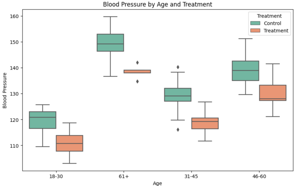
In the provided code, we are stratifying the population based on different age groups and then assigning treatment or control groups within each stratum.

1. ’18-30′ Age Group: For individuals aged between 18 and 30, we want to balance the treatment and control groups, so we use a 50-50 split. This ensures that within this age group, half of the individuals receive treatment, and the other half serve as the control group.
2. ’31-45′ Age Group: For individuals aged between 31 and 45, we assign a different split. In this case, we have a 30-70 split. This means that a smaller proportion (30%) of individuals in this age group receive treatment, while a larger proportion (70%) serve as the control group.
3. ’46-60′ Age Group: For individuals aged between 46 and 60, we assign an even more skewed split towards the control group. We use a 20-80 split, meaning that only 20% of individuals in this age group receive treatment, while 80% serve as the control group.
4. ’61+’ Age Group: Finally, for individuals aged 61 and above, we have the most skewed split towards the control group. We use a 10-90 split, where only 10% of individuals in this age group receive treatment, while 90% serve as the control group.

The rationale behind these varying splits is to ensure that within each age stratum, the treatment and control groups are balanced according to the chosen probabilities. This accounts for potential differences in treatment effects across different age categories and allows for more precise analysis by controlling for the influence of age as a covariate. Stratification helps prevent bias and ensures that comparisons between treatment and control groups are meaningful within each age stratum.

Balancing covariates through techniques mentioned above helps reduce bias by ensuring that treatment and control groups are comparable with respect to the relevant covariates. This improves the validity of the causal inference drawn from the analysis.

Conclusion.

In this blog post, we explored the significance of treatment group and control group in causal analysis. The treatment group represents individuals who are exposed to a specific treatment or intervention, while the control group consists of individuals who do not receive the treatment and serve as a baseline for comparison.

We discussed the importance of randomization in assigning individuals to treatment and control groups. Randomization ensures that participants have an equal chance of being assigned to either group, minimizing selection bias and allowing for unbiased estimation of the treatment effect. Randomization helps create comparable groups, making it more likely that any observed differences in outcomes between the groups are due to the treatment rather than pre-existing characteristics.

Additionally, we delved into the concept of covariates, which are factors that may influence both the treatment assignment and the outcome. Covariates can include demographic information, medical history, or other relevant factors. Balancing covariates between treatment and control groups is crucial to ensure a fair comparison and reduce confounding. Techniques such as matching, stratification, and regression adjustment can be employed to achieve balance and improve the accuracy of causal inference.

By understanding the role of treatment group and control group, the assignment of individuals, the role of randomization, and the importance of balancing covariates, we gain valuable insights into the process of conducting causal analysis. Considering these factors enhances the validity of causal inferences and strengthens the conclusions drawn from the analysis.

In our future posts, we will dive deeper into the counterfactual question and explore sensitivity analysis, which further expands our understanding of the treatment and control groups and their impact on causal analysis. Stay tuned for more insights on this fascinating topic!