Structure

1. What are confounding variables ?
2. Importance of identifying the confounders
3. Confounding bias and ways of removing it
4. Unraveling Simpson’s Paradox: The Impact of Confounders on Correlation and Causation
5. Mitigating the Influence of Confounders through Adjustment Formulae
6. Conclusion

Introduction

Today, we’ll embark on a journey to unravel the mysteries of confounding and understand its significant role in causal inference. To start, let’s dive into a simple and relatable example: a beachside shop that sells both ice creams and summer hats. During the scorching summer days, the shop owner notices an intriguing trend – a strong positive correlation between the sales of ice creams and summer hats. It seems that on days when more ice creams are sold, more summer hats fly off the shelves as well.

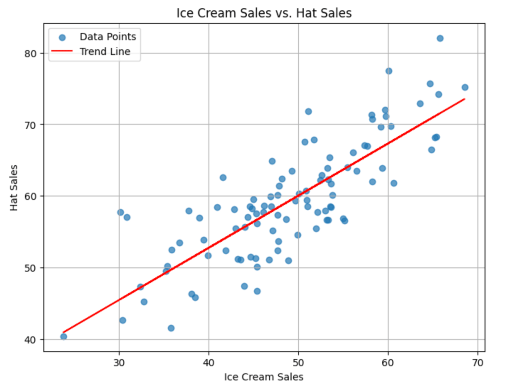
At first glance, one might assume a direct causal relationship between these two items – selling more ice creams causes an increase in summer hat sales, or vice versa. However, as we delve deeper into the underlying factors influencing this pattern, we come across a lurking variable that plays a pivotal role – the temperature. On hot summer days, people are naturally drawn to buy both ice creams and summer hats to beat the heat and enjoy the sunshine. In this scenario, the temperature acts as a confounding variable, affecting both ice cream and summer hat sales independently.

As we explore the concept of confounding further, we will uncover its potential to lead us astray when estimating causal effects in various scenarios. Confounding variables can introduce biases in our analysis, leading to incorrect conclusions about cause-and-effect relationships. Join us on this enlightening journey as we learn about the intricacies of confounding, its implications in causal analysis, and how to tackle it to obtain accurate and meaningful insights. So, let’s unravel the mysteries of confounding and enhance our understanding of causal inference together!

Importance of identifying the confounders

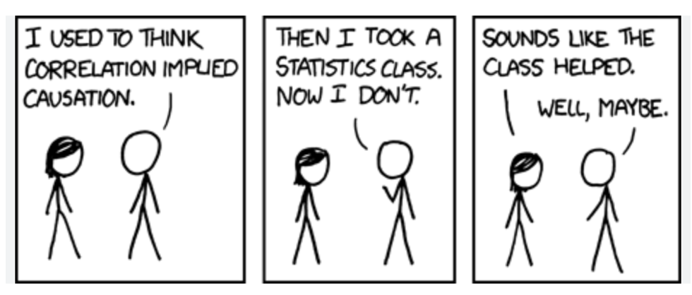
“Correlation is not causation” is a well-known phrase that serves as a poignant reminder of the potential pitfalls in making causal inferences solely based on observed associations. Let’s explore this idea through an example. Consider a study that examines the relationship between reading ability and shoe size in a group of students. Surprisingly, the study finds a strong positive correlation between these two variables – students with larger shoe sizes tend to have better reading skills. However, it would be misguided to conclude that bigger feet somehow enhance reading abilities or vice versa.

In this example, the concept of confounding comes into play. The lurking variable here is age. As students grow older, both their shoe sizes and reading abilities tend to increase. Age acts as a confounder, influencing both shoe size and reading ability independently. Therefore, the observed correlation between shoe size and reading ability is not indicative of a causal relationship between the two. Instead, it underscores the importance of carefully considering potential confounding factors before drawing any causal conclusions.

The phrase “correlation is not causation” serves as a cautionary reminder to remain vigilant in distinguishing between mere associations and genuine causal relationships. Without accounting for confounding variables, we risk falling prey to erroneous conclusions and misinterpretations of data. As we delve deeper into the realms of causal analysis, it becomes evident that understanding and addressing confounding is essential to unraveling the true cause-and-effect dynamics hidden within our observations.

Confounding bias and ways of removing it

Confounding bias poses a significant challenge in causal analysis, as it can lead to misleading conclusions and inaccurate assessments of the true causal relationship between a treatment and an outcome. A classic example of confounding bias arises when evaluating the efficacy of a new drug. Suppose the drug is primarily prescribed to older individuals, who are at higher risk for the targeted disease. Here, age acts as the confounder, influencing both the prescription of the drug and the likelihood of experiencing the disease outcome. Consequently, any adverse outcome in health among patients taking the drug could be mistakenly attributed to the drug’s effects, when in reality, it might be due to the age-related risk factors.

To disentangle the genuine impact of the new drug from the confounding effect of age, randomized controlled trials (RCTs) offer a powerful solution. In RCTs, patients are randomly assigned to either the treatment group, receiving the new drug, or the control group, receiving a placebo or standard treatment. Randomization ensures that potential confounders, like age, are evenly distributed among the groups, eliminating the bias that might have skewed the results in observational studies. By comparing the outcomes of both groups, researchers can confidently identify the true causal effect of the drug, making informed decisions about its efficacy and safety. Randomization helps to overcome confounding bias and strengthens the validity of causal analysis, providing more reliable evidence for medical practitioners and researchers.

Unraveling Simpson’s Paradox: The Impact of Confounders on Correlation and Causation

The well-known adage “correlation does not imply causation” reminds us that just because two variables are correlated, it doesn’t necessarily mean that one causes the other. This is especially true when confounding variables come into play, causing a spurious correlation or even a reversal of the direction of the association.

Simpson’s paradox is a classic example that exemplifies this phenomenon. It occurs when the relationship between two variables changes when a third variable, a confounder, is not taken into account. The confounding variable influences both the correlated variables, leading to a misleading overall conclusion.

Consider the pass percentage of female and male students in a semester.

	Female students	Male Students
Semester Pass percentage	78% ( 78/100)	81% ( 81/100)

At first glance, we observe that male students have a slightly higher pass percentage, seemingly indicating better academic performance. However, upon closer examination, we discover that the elective choices of students play a significant role.

	Female students	Male Students
Elective A ( Easy elective)	92% ( 23/25)	87% ( 67/77)
Elective B ( Tough elective)	73% ( 55/75)	61% ( 14/23)

When we analyze the pass percentages for each elective separately, we find that female students outperform male students in both difficult and easy electives. This means that, in reality, female students perform better in each category. However, the composition of elective choices creates an illusion of male students having an advantage in the overall results. Female students tend to opt for more challenging electives with lower pass rates, while male students prefer easier electives with higher pass rates. This disparity in the choice of electives is what creates the illusion of better performance of male students than that of the female students.

This example illustrates the importance of considering confounders in causal analysis. Failing to account for confounding variables can lead to erroneous conclusions and the misinterpretation of correlations. In this case the confounding variable is the choice of electives.The causal graph in this case is as represented below

A more equitable comparison in this case were to first condition on the electives and then compare the results of both male and female students. This entails considering the students who take the same elective as a group and then comparing the pass percentage of the male and female students within these groups. For example take students who take elective A, and then compare the pass percentage of male and female students ( 87% v/s 92% ). This is the essence of one of the methodologies to address Simpson’s paradox called the adjustment formulae. Let us look at the intuition behind the adjustment formulae next.

Mitigating the Influence of Confounders through Adjustment Formulae

In our earlier example, we delved into the intricacies of Simpson’s Paradox, where a seemingly straightforward comparison between the overall pass percentages of female and male students (78% vs. 81%) revealed a nuanced distortion. This distortion arose from the fact that female students disproportionately opted for more challenging courses, thus affecting their overall pass rate. The pivotal question that emerges is how to render this comparison more equitable, while factoring in the complexities introduced by confounding variables.

To address this quandary, let’s embark on a hypothetical scenario: envisage a student population entirely comprised of females. Within this context, the dynamics of the study population undergo a transformation. In the original scenario, the proportion of female students taking the demanding elective course was 77%, while the proportion opting for the less challenging course stood at 24%. We can now recalculate the overall pass percentage for female students using an alternative approach:

Overall Pass Percentage of Females = Pass Percentage in Demanding Course × Proportion of Females in Demanding Course + Pass Percentage in Less Challenging Course × Proportion of Females in Less Challenging Course

With calculations in mind, this results in:

Overall Pass Percentage of Females = 73% × 77% + 92% × 24% = 78%

Now, let’s transport ourselves to a hypothetical scenario where the entire student population consists solely of females. Although the individual pass percentages for the distinct courses remain unchanged (73% and 92%), what does undergo modification is the relative frequency or proportion of students opting for each course. With all students being females, the proportion of students enrolling in the demanding course would become (75 + 23)/200 = 49%. Similarly, the frequency of female students enrolling in the less challenging course would be (77 + 25)/200 = 51%.

In light of this adjustment, the recalculated overall pass percentage for the hypothetical all-female student population becomes:

Overall Pass Percentage (All-Female Scenario) = 73% × 49% + 92% × 51% ≈ 83%

Similarly the overall pass percentage if we consider all students be males would be

Overall Pass Percentage (All-male Scenario) = 62% × 49% + 87% × 51% ≈ 75%

Now these are comparable numbers which clearly indicate that female pass percentage is far better than the male pass percentage. The revised formulae which we used above is called the adjustment formulae.

This exercise showcases the influence of confounders on causal inferences and illustrates how adjustments, akin to this hypothetical scenario, can be applied to mitigate their impact. By understanding and effectively addressing confounding variables, we can attain a clearer and more accurate representation of the true relationships underlying the data.

Conclusion

In conclusion, our journey through the intricate landscape of confounding has unveiled a fundamental truth: causation is not correlation. We’ve delved into the nuances of confounding variables, those sneaky influencers that can distort the apparent relationship between our variables of interest. The adjustment formulae have emerged as our trusty tools, helping us navigate the labyrinth of observational data by accounting for these confounders.

Understanding the distinction between causation and correlation is paramount in unraveling the true nature of relationships within data. Confounding variables, often hidden in the shadows, can lead us astray if not properly acknowledged and addressed. The adjustment formulae act as our guiding light, allowing us to discern the genuine causal effects from mere associations.

As we part ways with confounding, let’s carry forth this wisdom: in the pursuit of understanding causation, we must tread carefully, armed with the knowledge that correlation does not imply causation. By diligently adjusting for confounders, we can unearth the threads of true causation, weaving a clearer narrative in the intricate tapestry of observational analysis.