

”Prototyping is the conversation you have with your ideas”
Tom Wujec
This is the fifth part of the series where we see our theoretical foundation on machine translation come to fruition. This series comprises of 8 posts.
- Understand the landscape of solutions available for machine translation
- Explore sequence to sequence model architecture for machine translation.
- Deep dive into the LSTM model with worked out numerical example.
- Understand the back propagation algorithm for a LSTM model worked out with a numerical example.
- Build a prototype of the machine translation model using a Google colab / Jupyter notebook.( This post)
- Build the production grade code for the training module using Python scripts.
- Building the Machine Translation application -From Prototype to Production : Inference process
- Build the machine translation application using Flask and understand the process to deploy the application on Heroku
In the previous 4 posts we understood the solution landscape for machine translation ,explored different architecture choices for sequence to sequence models and did a deep dive into the forward pass and back propagation algorithm for LSTMs. Having set a theoretical foundation on the application, it is time to build a prototype of the machine translation application. We will be building the prototype using a Google Colab / Jupyter notebook.
Building the prototype
The prototype building phase will consist of the following steps.
- Loading the raw data
- Preprocessing the raw data for machine translation
- Preparing the train and test sets
- Building the encoder – decoder architecture
- Training the model
- Getting the predictions
Let us get started in building the prototype of the application on a notebook
Downloading the raw text
Let us first grab the raw data for this application. The data can be downloaded from the link below.
http://www.manythings.org/anki/deu-eng.zip
This is also available in the github repository. The raw text consists of English sentences paired with the corresponding German sentence. Once the data text file is downloaded let us upload the data in our Google drive. If you do not want to do the prototype in Colab, you can download it in your local drive and then use a Jupyter notebook also for the purpose.
Preprocessing the text
Before starting the processes, let us import all the packages we will be using for the process
import string
import re
from numpy import array, argmax, random, take
from numpy.random import shuffle
import pandas as pd
from tensorflow.keras.models import Sequential
from tensorflow.keras.layers import Dense, LSTM, Embedding, RepeatVector
from tensorflow.keras.preprocessing.text import Tokenizer
from tensorflow.keras.callbacks import ModelCheckpoint
from tensorflow.keras.preprocessing.sequence import pad_sequences
from tensorflow.keras.models import load_model
from tensorflow.keras import optimizers
import matplotlib.pyplot as plt
% matplotlib inline
pd.set_option('display.max_colwidth', 200)
from pickle import dump
from unicodedata import normalize
from tensorflow.keras.models import load_model
The raw text which we have downloaded needs to be opened and progressively preprocessed through series of processing steps to ultimately get the train and test set which we require for building our models. Let us first define the path for the text, so as to take it from the google drive. This path has to be changed by you based on the path in which you load the data
# Define the path to the raw data set
fileurl = '/content/drive/My Drive/Bayesian Quest/deu.txt'
Once the path is defined, let us read the text data.
# open the file
file = open(fileurl, mode='rt', encoding='utf-8')
# read all text
text = file.read()
The text which is read from the text file would be in the format shown below
text[0:200]

From the output we can see that each record is seperated by a line (\n) and within each record the data we want is seperated by tabs (\t).So we can first split each record on new lines (\n) and after that each line we split on the tabs (\t) to get the data in the format we want
# Split the text into individual lines
lines = text.strip().split('\n')
# Splitting each line based on tab spaces and creating a list
lines = [line.split('\t') for line in lines]
# Visualizing first 5 lines
lines[0:5]

We can see that the processed records are stored as lists with each list containing an enlish word, its German translation and some metadata about the data. Let us store these lists as an array for convenience and then display the shape of the array.
# Storing the lines into an array
mtData = array(lines)
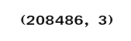
# Displaying the shape of the array
print(mtData.shape)
All the above steps we can represent as a function. Let us construct the function which will be used to load the data and do basic preprocessing of the data.
# function to read raw text file
def read_text(filename):
    # open the file
    file = open(filename, mode='rt', encoding='utf-8')
    # read all text
    text = file.read()

    # Split the text into individual lines
    lines = text.strip().split('\n')
    # Splitting each line based on tab spaces and creating a list
    lines = [line.split('\t') for line in lines]

    file.close()
    return array(lines)
We can call the function to load the data and convert it into an array of English and German sentences. We can also see that the raw data has more than 200,000 rows and three columns. We dont require the third column and therefore we can eliminate them. In addition processing all rows would also be computationally expensive. Let us take the first 50000 rows. However this decision is left to you on how many rows you want based on the capacity of your machine.
# Reading the data using the function
mtData = read_text(fileurl)
# Taking only 50000 rows of data
mtData = mtData[:50000,:2]
print(mtData.shape)
mtData[0:10]

With the array format, the data is in a neat format with the first column being English and the second one the corresponding German sentence. However if you notice the text, there are lot of punctuations and other characters which are unwanted. We also need to standardize the text to lower case. Let us now crank up our cleaning process. The following are the processes which we will follow
- Normalize all unicode characters,which are special characters found in a language, to its corresponding ascii format. We will be using a library called ‘unicodedata’ for this normalization.
- Tokenize the string to individual words
- Convert all the characters to lower case
- Remove all punctuations from the text
- Remove all non alphabets from text
Since there are multiple processes involved we will be wrapping all these processes in a function. Let us look at the code which implements this.
# Cleaning the document for all unwanted characters

def cleanDocs(lines):
  cleanArray = list()
  for docs in lines:
    cleanDocs = list()
    for line in docs:
      # Normalising unicode characters
      line = normalize('NFD', line).encode('ascii', 'ignore')
      line = line.decode('UTF-8')
      # Tokenize on white space
      line = line.split()
      # Removing punctuations from each token
      line = [word.translate(str.maketrans('', '', string.punctuation)) for word in line]
      # convert to lower case
      line = [word.lower() for word in line]
      # Remove tokens with numbers in them
      line = [word for word in line if word.isalpha()]
      # Store as string
      cleanDocs.append(' '.join(line))
    cleanArray.append(cleanDocs)
  return array(cleanArray)
The input to the function is the array which we created in the earlier step. We first initialize some empty lists to store the processed text in Line 3.
Lines 5 – 7, we loop through each row ( docs) and then through each column (line) of the row. The first process is to normalize the special characters . This is done through the normalize function available in the ‘unicodedata’ package. We use a normalization method called ‘NFD’ which maintains the same form of the characters in lines 9-10. The next process is to tokenize the string to individual words by applying the split() function in line 12. We then proceed to remove all unwanted punctuations using the translate() function in line 14 . After this process we convert the text to lower case and then retain only the charachters which are alphabets using the isalpha() function in lines 16-18. We join the individual columns within a row using the join() function and then store the processed row in the ‘cleanArray’ list in lines 20-21. The final output after the whole process looks quite clean and is ready for further processing.
# Cleaning the sentences
cleanMtDocs = cleanDocs(mtData)
cleanMtDocs[0:10]

Nueral Translation Data Set Preperation
Now that we have completed the initial preprocessing, its now time to get closer to the core process. Let us first prepare the data sets in the required format we want for modelling. The various steps which we will follow for preparation of data set are
- Tokenizing the text and creating vocabulary dictionaries for English and German sentences
- Define the sequence length for both English and German text
- Encode the text sequences as integer sequences
- Split the data set into train and test sets
Let us see each of these processes
Tokenization and vocabulary creation
Tokenization is the process of splitting the string to individual unique words or tokens. So if the string is
"Hi I am enjoying this learning and I look forward for more"
The unique tokens vocabulary would look like the following
{'i': 1, 'hi': 2, 'am': 3, , 'enjoying': 4 , 'this': 5 , 'learning': 6 'and': 7, , 'look': 8 , 'forward': 9, 'for': 10, 'more': 11}
Note that only unique words are taken and each token is given an index which will come in handy when we encode the tokens in later steps. So let us go ahead and prepare the tokens. Please note that we will be creating seperate vocabulary for English words and German words.
# Instantiating the tokenizer class
tokenizer = Tokenizer()
The function which does tokenization is the Tokenizer() class which could be imported from tensorflow.keras as shown above. The first step is to instantiate the Tokenizer() class. Next we will see how to fit text to the tokenizer object we created.
# Fit the tokenizer on the text
tokenizer.fit_on_texts(string)
Fitting the text is done using the fit_on_texts() method. This method splits the strings and then creates the vocabulary we saw earlier. Since these steps have to be repeated multiple times, let us package them as a function
# Function for creating tokenizers
def createTokenizer(lines):
    tokenizer = Tokenizer()
    tokenizer.fit_on_texts(lines)
    return tokenizer
Let us use the above function to create the tokenizer for English words and look at the total length of words in English
# Create English Tokenizer
eng_tokenizer = createTokenizer(cleanMtDocs[:,0])
eng_vocab_size = len(eng_tokenizer.word_index) + 1
print(eng_vocab_size)

We can see that the length of the English vocabulary is 6255. This is after we incremented the actual vocabulary size with 1 to account for any words which is not part of the vocabulary. Let us list down the first 10 words of the English vocabulary.
# Listing the first 10 items of the English tokenizer
list(eng_tokenizer.word_index.items())[0:10]

From the output we can see how the words are assigned an index value. Similary we will create the German vocabulary also
# Create German tokenizer
ger_tokenizer = createTokenizer(cleanMtDocs[:,1])
# Defining German Vocabulary
ger_vocab_size = len(ger_tokenizer.word_index) + 1
Now that we have tokenized the German and English sentences, the next task is to define a standard sequence length for these languges
Define Sequence lengths for German and English sentences
From our earlier introduction on sequence models, we know that we need data in sequences. A prerequisite in building sequence models is the sequences to be of standard lenght. However if we look at our corpus of both English and German sentences the lengths of each sentence will vary. We need to adopt a strategy for standardizing this length. One common strategy would be to adopt the maximum length of all the sentences as the standard sequence. Sentences which will have length lesser than the maximum length will have its indexes filled with zeros.However one pitfall of this strategy is, processing will be expensive. Let us say the length of the biggest sentence is 50 and most of the other sentences are of length ranging from 8 to 12. We have a situation wherein for just one sentence we unnecessarily increase the length of all other sentences by filling dummy values. When data sets become large, having all sentences standardized to the longest sentence will make the computation expensive.
To get over such issues we will adopt a strategy of finding a length under which majority of the sentences fall. This can be done by taking a high quantile value under which majority of the sentence lengths fall.
Let us implement this strategy. To start off we will have to count the lengths of all the sentences in the corpus
# Create an empty list to store all english sentence lenghts
len_english = []
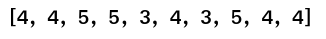
# Getting the length of all the English sentences
[len_english.append(len(line.split())) for line in cleanMtDocs[:,0]]
len_english[0:10]

In line 2 we first created an empty list 'len_english'. Next we iterated through all the sentences in the corpus and found the length of each of the sentences and then appended each sentence lengths to the list we created, line 4.
Similarly we will create the list of all German sentence lenghts.
len_German = []
# Getting the length of all the English sentences
[len_German.append(len(line.split())) for line in cleanMtDocs[:,1]]
len_German[0:10]
After getting a distribution of all the lengths of English sentences, let us find the quantile value at 97.5% under which majority of the sentences fall.
# Find the quantile length
engLength = np.quantile(len_english, .975)
engLength

From the quantile value we can see that a sequence length of 5.0 would be a good value to adopt as majority of the sentences would fall within this length. Similarly let us calculate for the German sentences also.
# Find the quantile length
gerLength = np.quantile(len_German, .975)
gerLength

We will be using the sequence lengths we have calculated in the next process where we encode the word tokens as sequences of integers.
Encode the sequences as integers
Earlier we tokenized all the unique words and created vocabulary dictionaries. In those dictionaries we have a mapping of the word and an integer value for the word. For example let us display the first 5 tokens of the english vocabulary
# First 5 tokens and its integers of English tokenizer
list(eng_tokenizer.word_index.items())[0:5]

We can see that each tokens are associated with an integer value . In our sequence model we will be using the integer values instead of the tokens themselves. This process of converting the tokens to its corresponding integer values is called the encoding. We have a method called ‘texts_to_sequences’ in the tokenizer() to convert the tokens to integer sequences.
The standard length of the sequence which we calculated in the previous section will be the length of each of these integer encoding. However what happens if a sentence string has length more than the the standard length ? Well in that case the sentence string will be curtailed to the standard length. In the case of a sentence having length less than the standard length, the additional lengths will be filled with zeros. This process is called padding.
The above two processes will be implemented in a function for convenience. Let us look at the code implementation.
# Function for encoding and padding sequences

def encode_sequences(tokenizer,length, lines):
    # Sequences as integers
    X = tokenizer.texts_to_sequences(lines)
    # Padding the sentences with 0
    X = pad_sequences(X,maxlen=length,padding='post')
    return X
The above function takes three variables
tokenizer : Which is the language tokenizer we created earlier
length : The standard length
lines : Which is our data
In line 5 each line is converted to sequenc of integers using the 'texts_to_sequences' method and then padded using pad_sequences method, line 7. The parameter value of padding = 'post' means that the zeros are added after the corresponding length of the sentence till the standard length is reached.
Let us now use this function to prepare the integer sequence data for both English and German sentences. We will split the data set into train and test sets first and then encode the sequences. Please remember that German sequences are our X variable and English sentences are our Y variable as we are translating from German to English.
# Preparing the train and test splits
from sklearn.model_selection import train_test_split
# split data into train and test set
train, test = train_test_split(cleanMtDocs, test_size=0.1, random_state = 123)
print(train.shape)
print(test.shape)

# Creating the X variable for both train and test sets
trainX = encode_sequences(ger_tokenizer,int(gerLength),train[:,1])
testX = encode_sequences(ger_tokenizer,int(gerLength),test[:,1])
print(trainX.shape)
print(testX.shape)

Let us display first few rows of the training set
# Displaying first 5 rows of the traininig set
trainX[0:5]

From the visualization of the training set we can see the integer encoding of the sequences and also padding of the sequences . Similarly let us repeat the process for English sentences also.
# Creating the Y variable both train and test
trainY = encode_sequences(eng_tokenizer,int(engLength),train[:,0])
testY = encode_sequences(eng_tokenizer,int(engLength),test[:,0])
print(trainY.shape)
print(testY.shape)

We have come to the end of the preprocessing steps. Let us now get to the heart of the process which is defining the model and then training the model with the preprocessed training data.
Nueral Translation Model Building
In this section we will look into the building blocks of the model. We will define the model structure in a function as shown below. Let us dive into details of the model
def defineModel(src_vocab,tar_vocab,src_timesteps,tar_timesteps,n_units):
    model = Sequential()
    model.add(Embedding(src_vocab,n_units,input_length=src_timesteps,mask_zero=True))
    model.add(LSTM(n_units))
    model.add(RepeatVector(tar_timesteps))
    model.add(LSTM(n_units,return_sequences=True))
    model.add(TimeDistributed(Dense(tar_vocab,activation='softmax')))
    # Compiling the model
    model.compile(optimizer = 'adam',loss='sparse_categorical_crossentropy')
    # Summarising the model
    model.summary()

    return model
In the second article of this series we were introduced to the encoder-decoder architecture. We will be manifesting the encoder architecture within this code block. From the above code uptill line 5 is the encoder part and the remaining is the decoder part.
Let us now walk through each layer in this architecture.
Line 2 : Sequential Class
As you know neural networks, work on the basis of various layers stacked one after the other. In Keras, representation of the model as a stack of layers is initialized using a class called Sequential(). The sequential class is usable for most of the cases except in cases where one has to share multiple layers or have multiple inputs and outputs. For the latter case the functional API in keras is used. Since the model we have defined is quite straight forward, using sequential class will suffice.
Line 3 : Embedding Layer
A basic requirement for a neural network model is the input to be in numerical format. In our case our inputs are text format. So we have to convert this text into some numerical features. Word embedding is a very effective way of representing the sequence of texts in the form of numbers ensuring that the syntactic relationship between words in the sequence is also maintained.
Embedding layer in Keras can be explained in simple terms as a look up dictionary between the unique words in the vocabulary and the corresponding vector of that word. The vector for each word which is the representation of the semantic similarity is learned during the training process. The Embedding function within Keras requires the following parameters vocab_size, embedding_size and sequence_length
Vocab_size : The vocab size is required to initialize the matrix of unique words and its corresponding vectors. The unique indexes of each word is initialized based on the vocab size. Let us look at an example to illustrate this.
Suppose there are two sentences with the following words
‘Embedding gets the semantic relationship between words’
‘Semantic relationships manifests the context’
For demonstration purpose let us assume that the initial vector representation of these words are as shown in the table below.
| Index | Word | Vector |
| 0 | Embedding | [0.02 , 0.01 , 0.12] |
| 1 | gets | [0.21 , 0.41 , 0.52] |
| 2 | the | [0.22 , 0.61 , 0.02] |
| 3 | semantic | [0.71 , 0.01 , 0.32] |
| 4 | Relationship | [0.85 ,-0.23 , -0.52] |
| 5 | between | [0.21 , -0.45 , 0.62] |
| 6 | words | [-0.29 , 0.91 , 0.052] |
| 7 | manifests | [0.121 , 0.401 , 0.352] |
| 8 | context | [0.721 , 0.531 , -0.592] |
Let us understand each of the parameters of the embedding layer based on the above table. In our model the vocab size for the encoder part is the German vocabulary size. This is represented as src_vocab, which stands for source vocabulary. For the toy example we considered, our vocab size is 9 as there are 9 unique words in the above table.
embedding size : The second parameter which needs to be supplied is the embedding size. This represents the size of the vector for each word in the matrix. In the example matrix shown above the vector size is 3. The size of the embedding vector is a parameter which can be altered to get the right semantic relationship between the sequences of words in the sentence
sequence length : The sequence length represents the number of words which are required in each input sentence. As seen earlier during preprocessing, a pre-requisite for the LSTM layer was for the length of sequences to be standardized. If a particular sequence has less number of words than the sequence length, it was padded with dummy vectors so that the length was standard. For illustration purpose let us assume that the sequence length = 10. The representation of these two sentence sequences in the vector form will be as follows
[Embedding, gets, the ,semantic, relationship, between, words] => [[0.02 , 0.01 , 0.12], [0.21 , 0.41 , 0.52], [0.22 , 0.61 , 0.02], [0.71 , 0.01 , 0.32], [0.85 ,-0.23 , -0.52], [0.21 , -0.45 , 0.62], [-0.29 , 0.91 , 0.052], [0.00 , 0.00, 0.00], [0.00 , 0.00, 0.00]]
[Semantic, relationships, manifests ,the, context] => [[0.71 , 0.01 , 0.32], [0.85 ,-0.23 , -0.52], [0.121 , 0.401 , 0.352] ,[0.22 , 0.61 , 0.02], [0.721 , 0.531 , -0.592], [0.00 , 0.00, 0.00], [0.00 , 0.00, 0.00], [0.00 , 0.00, 0.00], [0.00 , 0.00, 0.00], [0.00 , 0.00, 0.00]]
The last parameter mask_zero = True is to inform the Model that some part of the data is padding data.
The final output from the embedding layer after providing all the above inputs will be a three dimensional matrix of the following shape (No. of samples ,sequence length , embedding size). Let us view this pictorially

As seen from the above figure, let each rectangular block represent the vector representation of a word in the sequence. The depth of the block will be the embedding size dimensions. Multiple words along the ‘X’ axis will form a sequence and multiple such sequences along the ‘Y’ axis will represent the number of examples we have in the corpora.
Line 4 : Sequence to sequence Layer (LSTM)
The next layer in the model is the sequence to sequence layer which in our case is a LSTM. We discussed in detail the dynamics of the LSTM layer in the third and fourth articles of the series. The number of hidden units is defined as a parameter when defining the LSTM unit.
Line 5 : Repeat Vector
In our machine translation application, we need to produce output which is equal in length with the standard sequence length of the target language ( English) . However our input at the encoder phase is equal in length to the source sequence ( German ). We therefore need a mechanism to map the output from the encoder phase to the number of sequences of the decoder phase. A ‘Repeat Vector’ is that operation which maps the input sequences (German sequence) to that of the output sequences ( English sequence). The below figure gives a pictorial representation of the operation.

As seen in the figure above we have to match the output from the encoder and the decoder. The sequence length of the encoder will be equal to the source sequence length ( German) and the length of the decoder will have to be the length of the target sequence ( English). Repeat vector can be described as a trick to match them. The output vector of the encoder where the information of the complete sequence is encoded is repeated in this operation. It is important to note that there are no weights and parameters in this operation.
Line 6 : LSTM Layer ( with return sequence is true)
The next layer is another LSTM unit. The dynamics within this unit is the same as the previous LSTM unit. The only difference in the output. In the previous LSTM unit we never had any output from each of the sequences. The output sequences is controlled by the parameter return_sequences. By default it is ‘False’. However in this case we have specified the return_sequences = True . This means that we need to have an output from each of the sequences. When we keep the return_sequences = False only the last sequence will have an output.
Line 7 : Time Distributed – Dense Layer with Softmax activation
This is the final layer of the network. This layer receives the output from the pervious LSTM layer which has outputs equal to the target sequence. Each of these sequences are then connected to a dense layer or a fully connected layer. Dense layer in Keras is synonymous to the dot product of the output and weight matrix along with addition of the bias term.
Dense = dot(Wy , Y) + by
Wy = Weight matrix of the Dense layer
Y = Output from each of the LSTM sequence
by = bias term for each sequence
After the dense operation, the resultant vector is taken through a softmax layer which converts the output to a probability distribution around the vocabulary of the target language. Another term to note is the command Time distributed. This implies that each sequence output which we get out of the LSTM layer has to be applied to a separate dense operation and a subsequent Softmax layer. So at the end of all the operation we will get a probability distribution around the target vocabulary from each of the output

Line 9 Optimizer
In this layer the optimizer function and the loss functions are defined. The loss function we have defined is sparse_cross entropy, which is beneficial from a training perspective. If we use categorical_cross entropy we would require one hot encoding of the output matrix which can be very expensive to train given the huge size of the target vocabulary. Sparse_cross entropy gives us a great alternate.
Line 11 Summary
The last line is the summary of the model. Let us try to unravel each of the parameters of the summary level based on our understanding of the LSTM

The summary displays the model layer by layer the way we built it. The first layer is the embedding layer where the output shape is (None,6,256). None stands for the number of examples we have. The other two are the length of the source sequence ( src_timesteps = gerLength) and the embedding size ( 256 ).
Next we applied a LSTM layer with 256 hidden units which is represented as (None , 256 ). Please note that we will only have one output from this LSTM layer as we have not specified return_sequences = True.
After the single LSTM layer we have the repeat vector operations which copies the single output of the LSTM to a length equal to the target language length (engLength = 5).
We have another LSTM layer after the repeat vector operation. However in this LSTM layer we have defined the output as return_sequences=True . Therefore we have outputs of 256 units each for each of the sequence resulting in the output dimension of ( None, 5 , 256).
Finally we have the time distributed dense layer. We earlier saw that the time distributed dense layer will be a dense operation on each of the time sequence. Each sequence will be of the form Dense = dot(Wy , Y) + by. The weight matrix Wy will have a dimension of (256,6225 ) where 6225 is the dimension of the target vocabulary ( eng_vocab_size = 6225). Y is the output from each of the LSTM layer from the previous layer which has a dimension ( 1, 256 ). So the dot product of both these matrices will be
[ 1, 256 ] x [256,6225] = >> [1, 6225]
The above is for one time step. When there are 5 time steps for the target language we will get a dimension of ( None , 5 , 6225)
Model fitting
Having defined the model and the optimization function its time to fit the model on the data.
# Fitting the model
checkpoint = ModelCheckpoint('model1.h5',monitor='val_loss',verbose=1,save_best_only=True,mode='min')
model.fit(trainX,trainY,epochs=50,batch_size=64,validation_data=(testX,testY),callbacks=[checkpoint],verbose=2)
The initiation of both the forward and backward propagation is through the model.fit function. In this function we provide the inputs (trainX and trainY), the number of epochs , the batch size for each pass of the optimizing function and also the validation set. We also define the checkpointing to save our models based on the validation score. The model fitting process or training process is a time consuming step. During the train phase the forward pass, error identification and the back propogation processes will kick in.
With this we come to the end of the training process. Let us look back and summarize the model architecture to get a big picture of the process.
Model Big picture
Having seen the model components, let us now get a big picture as to the whole process and how the forward and back propagation work together to learn the required parameters from the data.

The start of the process is the creation of the features for the model namely the embedding layer. The inputs for the input layer are the source vocabulary size, embedding size and the length of the sequences. The output we get out of this is a three dimensional matrix with number of examples, sequence length and the embedding size as the three dimensions.
The embedding layer is then supplied to the first LSTM layer as input with each time step receiving an embedding layer . There will not be any output for each time step of the sequence. The only output will be from the last time step which is then given as input to the next LSTM layer. The number of time steps of the second LSTM unit will be the equal to length of the target language sequence. To ensure that the LSTM has inputs equal to the target sequences, the repeat vector function is used to copy the output from the previous LSTM layer to all the time steps of the second LSTM layer.
The second LSTM layer will given intermediate outputs for each of the time steps. Each of these outputs are then fed into a dense layer. The output of the dense layer will be a vector equal to the vocabulary length of the target language. This vector is then passed on to the softmax layer to convert it into a probability distribution around the target vocabulary. The output from the softmax layer, which is the prediction is compared with the actual label and the difference would be the error.
Once the error is generated, it has to be back propagated to all the parts of the network to get the gradients of each of the parameters. The error will start propagating first from the dense layer and then would propagate to each of the sequence of the second LSTM unit. Within the LSTM unit the error will start propogating from the last sequence and then will progressively move towards the first sequence. During the movement of the error from the last sequence to the first, the respective errors from each of the sequences are added to the propagated error so as to get the gradients. The final weight gradient would be sum of the gradients obtained from each of the sequence of the LSTM as seen from the numerical example on back propagation. The gradient with respect to each of the inputs will also be calculated by summing across all the time step. The sum total of the gradients of the inputs from the second LSTM layer will be propagated back to the first LSTM layer.
In the first LSTM layer, the gradient received from the top layer will be propagated from the last time sequence. The error propagates progressively through each time step. In this LSTM there will not be any error to be added at each sequence as there were no output for each of the sequence except for the last layer. Along with all the weight gradients , the gradient vector for the embedding vector is also calculated. All these operations are carried out for all the epochs and finally the model weights are learned, which help in the final prediction.
Once the training is over, we get the most optimised parameters inside the model object. This model object is then used to predict on the test data set. Let us now look at the prediction or inference phase of the process.
Inference Process
The proof of the pudding of the model we created is the predictions we get from a test set. Let us first look at how the predictions would be from the model which we just created
# Generating the predictions
prediction = model.predict(testX,verbose=0)
prediction.shape

We get the prediction from the model using model.predict() method with the test data as its input. The prediction we get would be of shape ( num_examples, target_sequence_length,target_vocabulary_size). Each example will be a sequence of probability distribution around the target vocabulary. For each sequence the predicted word would be the index of the vocabulary where the probability is the greatest. Let us demonstrate this with a figure.
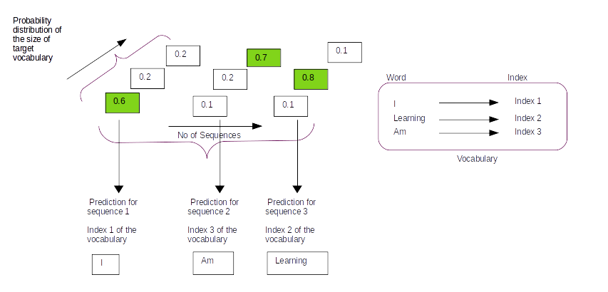
Let us assume that the vocabulary has only three words [ I , Learning , Am] with indexes as [1,2,3] respectively. On predicting with the model we will get a probability distribution on each sequence as shown in the figure above. For the first sequence the probability for the first index word is 0.6 and the other two are 0.2 and 0.2 resepectively. So from the probability distribution the word in the first index has the largest probability and that will be the predicted word for that sequence. So based on the index with the maximum probability for the entire sequence we get the predictions as [1,3,2] which translates to [I , Am, Learning] as per the vocabulary.
To get the index of each of the sequences, we use a function called argmax(). This is how the code to get the indexes of the predictions will look
# Getting the prediction index along the last axis ( Vocabulary size axis)
predIndex = [argmax(vector,axis = -1) for vector in prediction]
predIndex[0:3]

In the above code axis = -1 means that the argmax has to be taken on the last dimension of the prediction which is along the vocabulary dimension. The prediction we get will be in the form of sequences of integers having the same sequence length as the target vocabulary.
If we look at the first 3 predictions we can see that the predictions are integers which have to be converted to the corresponding words. This can be done using the tokenizer dictionary we created earlier. Let us look at how this is done
# Creating the reverse dictionary
reverse_eng = eng_tokenizer.index_word
The index_word, method of the tokenizer class generates the word for an input index. In the above step we have created a dictionary called reverse_eng which outputs a word when given an index. For a sequence of predictions we have to loop through all the indexes of the predictions and then generate the predicted words as shown below.
# Converting the tokens to a sentence
preds = []
for pred in predIndex[0]:
  if pred == 0:
        continue
  preds.append(reverse_eng[pred])
print(' '.join(preds))

In the above code block in line 2 we first initialized an empty list preds . We then iterated through each of the indexes in lines 3-6 and generated the corresponding word for the index using the reverse_eng dictionary. The generated words are finally appended to the preds list. We joined all the words in the list together get our predicted sentence.
Let us now package all the inference code we have seen so far into two functions.
# Creating a function for converting sequences
def Convertsequence(tokenizer,source):
    target = list()
    reverse_eng = tokenizer.index_word
    for i in source:
        if i == 0:
            continue
        target.append(reverse_eng[int(i)])
    return ' '.join(target)
The first function is to convert the sequence of predictions to a sentence.
# Function to generate predictions from source data
def generatePredictions(model,tokenizer,data):
    prediction = model.predict(data,verbose=0)
    AllPreds = []
    for i in range(len(prediction)):
        predIndex = [argmax(prediction[i, :, :], axis=-1)][0]
        target = Convertsequence(tokenizer,predIndex)
        AllPreds.append(target)
    return AllPreds
The second function is to generate predictions from the test set and then generate the predicted sentence. The first function we defined is used inside the generatePredictions function.
Now that we have understood how the predictions can be generated let us go ahead and generate predictions for the first 20 examples of the test set and evaluate the results.
# Generate predictions
predSent = generatePredictions(model,eng_tokenizer,testX[0:20,:])
for i in range(len(testY[0:20])):
    targetY = Convertsequence(eng_tokenizer,testY[i:i+1][0])
    print("Original sentence : {} :: Prediction : {}".format([targetY],[predSent[i]]))

From the output we can see that the predictions are pretty close in a lot of the examples. We can also see that there are some instances where the context is understood and predicted with different words like the examples below


There are also predictions which are way off the target


However considering the fact that the model we used was simple and the data set we used were relatively small, the model does a reasonably okay job.
Inference on your own sentences
Till now we predicted on the test set. Let us see how we can generate predictions from an input sentence we provide.
To generate predictions from our own input sentences, we have to first clean the input sentences and then tokenize them to transform it to the format the model understands. Let us look at the functions which does these tasks.
def cleanInput(lines):
    cleanSent = []
    cleanDocs = list()
    for docs in lines.split():
        line = normalize('NFD', docs).encode('ascii', 'ignore')
        line = line.decode('UTF-8')
        line = [line.translate(str.maketrans('', '', string.punctuation))]
        line = line[0].lower()
        cleanDocs.append(line)
    cleanSent.append(' '.join(cleanDocs))
    return array(cleanSent)
The first function is the cleaning function. This is an abridged version of the cleaning function we used for our original data set. The second function we will use is the encode_sequences function we used earlier. Using these functions let us go ahead and generate our predictions.
# Trying different input sentences
inputSentence = 'Es ist ein großartiger Tag' # It is a great day ?
The first sentence we will try is the German equivalent of 'It is a great day ?'.
Let us clean the input text first using the function we developed
# Clean the input sentence
cleanText = cleanInput(inputSentence)
Next we will encode this sentence into sequence of integers
# Encode the inputsentence as sequence of integers
seq1 = encode_sequences(ger_tokenizer,int(gerLength),cleanText)
Let us get our predictions and print them out
# Generate the prediction
predSent = generatePredictions(model,eng_tokenizer,seq1)

print("Original sentence : {} :: Prediction : {}".format([cleanText[0]],predSent))

Its not a great prediction isnt it ?? Let us try couple more sentences
inputSentence1 ='Heute wird es regnen' #  it's going to rain Today
inputSentence2 ='Ich habe im Radio gesprochen' # I spoke on the radio

for sentence in [inputSentence1,inputSentence2]:
  cleanText = cleanInput(sentence)
  seq1 = encode_sequences(ger_tokenizer,int(gerLength),cleanText)
  # Generate the prediction
  predSent = generatePredictions(model,eng_tokenizer,seq1)

  print("Original sentence : {} :: Prediction : {}".format([cleanText[0]],predSent))

We can see that the predictions on our own sentences are not promising .
Why is it that the test set gave us reasonable predictions and our own sentences are not giving good predicitons ? Well one obvious reason is that the distribution of words we used could be different from the distribution which was used for training. Besides,the model we used was a simple one and the data set also relatively small. All these could be the reasons for bad predictions on our own sentences. So how do we improve the quality of predictions ? There are different ways to do that. Let us see some of them.
- Use bigger data set for training and train for longer epochs.
- Change the model architecture. Experiment with different number of units and number of layers. Try variations like bidirectional LSTM
- Try out different regularization methods like drop out.
- Use attention mechanisms
There are different avenues for improvement. I would urge you to try out different choices and let me know how your fared.
Next Steps
Congratulations, we have successfully built a prototype for machine translation system. The next step in our journey is to convert this prototype into an application. We will address that in the next post.
Go to article 6 of this series : From prototype to production
You can download the notebook for the prototype using the following link
https://github.com/BayesianQuest/MachineTranslation/tree/master/Prototype
Do you want to Climb the Machine Learning Knowledge Pyramid ?
Knowledge acquisition is such a liberating experience. The more you invest in your knowledge enhacement, the more empowered you become. The best way to acquire knowledge is by practical application or learn by doing. If you are inspired by the prospect of being empowerd by practical knowledge in Machine learning, I would recommend two books I have co-authored. The first one is specialised in deep learning with practical hands on exercises and interactive video and audio aids for learning

This book is accessible using the following links
The Deep Learning Workshop on Amazon
The Deep Learning Workshop on Packt
The second book equips you with practical machine learning skill sets. The pedagogy is through practical interactive exercises and activities.

This book can be accessed using the following links
The Data Science Workshop on Amazon
The Data Science Workshop on Packt
Enjoy your learning experience and be empowered !!!!

It is a free course. Please reply me.
LikeLike